import numpy as np
import matplotlib.pyplot as plt
import longitudinal as lde
%matplotlib notebook
# Longitudinal Dynamics
Acceleration of Charged Particle
Modern accelerators use RF/SRF cavities as the accelerating device, as shown below.
 Usually TM010 mode of the cavity is used and the accelerating field is written as:
$E_0(s)$ is the field amplitude and $t$ is the time and the $\phi_0$ is the initial phase at $t=0$. The choise of the initial phase will be clear later when the beam travels through the cavity. The cavity is defined from the "potential of the field amplitude": $$V=\int_{-\infty}^{\infty}E_0(s)ds$$
However this is not the potential that the particle sees. Let assume a particle passing through a cavity, which has a 6D coordinate $(x, p_x, y, p_y, z=-\beta ct', \delta=\Delta p/p_0)$. Here $\beta=v/c$ and $t'$ is the arrival time difference with respective to the reference particle at observation time (the prime was added to separate from the clock time t). And we assume that the particle velocity does not change during passing through the cavity. We know that: $$ \frac{d\beta}{\beta} = \frac{1}{\beta^2\gamma^2} \frac{d\gamma}{\gamma} $$This is approximately true in the following two scenario:
- Particle is already relativistic ($\gamma \gg 1$)
- The energy gain in the cavity much smaller than the particle's momentum ($d\gamma \ll \beta\gamma$)
Within the cavity, if the reference particle arrives $s=0$ at $t_0$, the particle we consider is located at $s=\beta c (t-t_0)+z$ The energy gain of the particle, traveling through the field $E(s,t)$ is:
\begin{align} \Delta U&=q\int_{-\infty}^{\infty} E(s,t) ds \nonumber\\ &= q\int_{-\infty}^{\infty} E_0(s) \sin\left(\frac{\omega (s-z)}{\beta c}+\phi_s\right)ds \end{align}The $\phi_s$ absorbs the $t_0$ terms and becomes the synchronous phase. In usual cases of symmetric cavities, the envelope is an even function $E_0(s)=E_0(-s)$ Then the energy gain can be simplified as:
\begin{align} \Delta U &=q \int_{-\infty}^{\infty} E_0(s) \sin\left(\frac{\omega (s-z)}{\beta c}+\phi_s\right)ds \nonumber \\ &=q\left(\int_{-\infty}^{\infty} E_0(s) \cos\frac{\omega s}{\beta c} ds\right) \sin \left(\phi+\phi_s\right)\nonumber\\ &\equiv qVT\sin \phi \end{align}Here we use $\phi=\phi_s-\omega z/\beta c=\phi_s+\omega t'$ as the longitudinal coordinate for later convenience. Here we use 'cavity voltage' $V$ and the time transient factor $T$ of a RF cavity to replace the 'real voltage' seen by the beam. The time transient factor $T$ is defined as:
\begin{align} T=\frac {\int_{-\infty}^{\infty} E_0(s) \cos\frac{\omega s}{\beta c} ds} {\int_{-\infty}^{\infty} E_0(s) ds} \end{align}From now on, we will redefine the voltage $V$ as the real voltage seen by the beam, to avoid the appearance of the time transient factor in the below beam dynamics analysis.
For reference particle, the energy gain is simply as
\begin{align} \Delta U_0 = qV\sin \phi_s \end{align}So after passing the cavity, the change of the energy deviation from the reference particle $\Delta E=E-E_0$ is simply:
\begin{align} \Delta E|_1&=\Delta E|_0+\Delta U-\Delta U_0 \nonumber\\ &=\Delta E|_0 + qV \left(\sin \phi-\sin \phi_s\right) \end{align}The subscript 1 and 0 represent the value after and before the cavity respectively.
Dynamics in a Ring Accelerator
Longitudinal transfer map
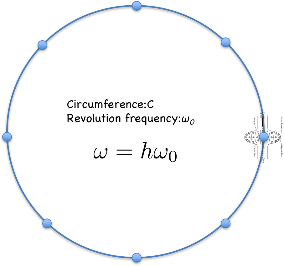
In a ring, there are one or several isolated locations to install the accelerating RF cavities. To synchronize with the beam arriving time of each revolution, the frequency of the RF must be multiple of the revolution frequency: $$f_{RF}=hf_0=h/T_0$$
$h$ is called harmonic number. For now let's assume only one cavity present in the ring.
If we describe the dynamics turn-by-turn and use the subscript $n$ to denote the the quantity before the entering the cavity for the $(n+1)^{th}$ time. Therefore we can write the energy change as:
\begin{equation} \Delta E_{n+1}= \Delta E_{n} + qV \left(\sin \phi_n-\sin \phi_s\right) \end{equation}Using the fact that:
\begin{equation} \delta=\frac{\Delta p}{p_0}=\frac{1}{\beta^2}\frac{\Delta E}{E_0} \end{equation}We get:
\begin{equation} \delta_{n+1}= \delta_{n} + \frac{qV}{\beta^2 E_0} \left(\sin \phi_n-\sin \phi_s\right) \end{equation}Now we need to establish the relation for the phase $\phi_n=\omega t$
\begin{align} \phi_{n+1} &=\phi_{n} + \omega T_0\eta\delta_{n+1} \nonumber\\ &=\phi_{n} + 2\pi h \eta \delta_{n+1} \end{align}Alternatively, we may write
\begin{align} \phi_{n+1} = \phi_{n} + \frac{2\pi h \eta}{\beta^2 E_0} \Delta E_{n+1} \end{align}Therefore the longitudinal dynamics is described by a map from $n^{th}$ to the ${n+1}^{th}$ using variable $(\delta, \phi)$:
\begin{align} \delta_{n+1}&=\delta_{n} + \frac{qV}{\beta^2 E_0} \left(\sin \phi_n-\sin \phi_s\right)\\ \phi_{n+1}&=\phi_{n} + 2\pi h \eta \delta_{n+1} \end{align}For the non zero $\phi_s$ indicates a net acceleration or deceleration in one turn to the reference particle. In electron storage rings the net acceleration is required to compensate the synchrotron radiation loss. In this case the $E_0$ and $p_0$ in of one turn is still constant.
In the case of synchrotron, the reference energy changes therefore using the variable $(\Delta E, \phi)$ is more convenient:
\begin{align} \Delta E_{n+1} &=\Delta E_{n} + qV \left(\sin \phi_n-\sin \phi_s\right)\\ \phi_{n+1} &= \phi_{n} + \frac{2\pi h \eta}{\beta^2 E_0} \Delta E_{n+1} \end{align}In either case, the Jacobian of the transfer map has determinant 1, due to the update of the phase relying on the new energy instead of the old one. Therefore under such map the phase space area $(\delta, \phi)$ or $(\Delta E, \phi)$ is conserved assuming the parameters are constant.
Let's look at the fix point of the phase space area, which transfers $(\delta, \phi)\rightarrow(\delta, \phi)$. It is easy to find that $(0,\phi_s)$ and $(0,\pi-\phi_s)$. We can explore the area at the vicinity of the fix points.
Let's consider the following example of a synchrotron (base on RHIC of BNL):
| Parameters | Value |
|---|---|
| Injecton energy | 20 GeV |
| Top energy | 250 GeV |
| Mass | 0.938 GeV |
| RF voltage | 5 MV |
| RF frequency | 28.15 MHz |
| Harmonic | 360 |
| $\alpha_c$ | 0.0018 |
The required energy gain per turn is $\Delta U < eV$ to compensate some energy loss. Which means the required synchrotron phase $\phi_s$ is: $$ \sin\phi_s = \Delta U/eV $$
In the following example, let's assume $\sin\phi_s = 0.5$. Therefore there are two solutions: $\phi_s = \pi/6$ or $\phi_s = 5\pi/6$. Let's consider a group of particles, who have same phase but different initial momentum deviations.
turns=2100
sin_phi_s=0.5
#phi_s=0
energy_list=[250e9,20e9]
mass=0.938e9
harm=360
voltage=5e6
mcf=0.0018
update_eta=True

#print(height)

# Vicinity of the pi-phi_s
fig,ax=plt.subplots(1,2,figsize=(10,4))

npar=5
result_g1=[]
for i in range(len(energy_list)):
    beam_energy=energy_list[i]
    gamma=beam_energy/mass
    eta=mcf-1/gamma/gamma
    beta=np.sqrt(1-1/gamma/gamma)
    phi_s=np.arcsin(sin_phi_s)
    yf=np.sqrt(np.cos(phi_s)-(np.pi-2*phi_s)*np.sin(phi_s)/2)
    height=2*np.sqrt(voltage/2/np.pi/beta/beta/beam_energy/harm/np.abs(eta))*yf

    initial_phi=np.ones(npar)*(np.pi-phi_s)
    initial_delta=np.linspace(height/npar, height*0.99, npar)
    temp=lde.longitudinal_evolve_delta(turns,
                                       initial_phi,
                                       initial_delta,
                                       sin_phi_s=sin_phi_s, alphac=mcf, E0_ini=beam_energy,
                                       mass=mass, e_volt=voltage, harm=harm,
                                       update_eta=update_eta
                                      )
    result_g1.append(temp)

# Vicinity of the phi_s

result_g2=[]
for i in range(len(energy_list)):
    beam_energy=energy_list[i]
    gamma=beam_energy/mass
    eta=mcf-1/gamma/gamma
    beta=np.sqrt(1-1/gamma/gamma)
    phi_s=np.arcsin(sin_phi_s)
    yf=np.sqrt(np.cos(phi_s)-(np.pi-2*phi_s)*np.sin(phi_s)/2)
    height=2*np.sqrt(voltage/2/np.pi/beta/beta/beam_energy/harm/np.abs(eta))*yf
    ax[i].set_ylim([-2*height,2*height])
    initial_phi=np.ones(npar)*(phi_s)
    initial_delta=np.linspace(0, height*0.99, npar)
    temp=lde.longitudinal_evolve_delta(turns,
                                       initial_phi,
                                       initial_delta,
                                       sin_phi_s=sin_phi_s, alphac=mcf, E0_ini=beam_energy,
                                       mass=mass, e_volt=voltage, harm=harm,
                                       update_eta= update_eta
                                      )
    result_g2.append(temp)


for i in range(2):
    ax[i].set_aspect('auto')
    ax[i].set_title("{} GeV".format(energy_list[i]/1e9))
    ax[i].set_xlabel('Phase [rad]')

    ax[i].set_xlim([-np.pi,2*np.pi])

    ax[i].set_prop_cycle(plt.cycler('color', plt.cm.Oranges(np.linspace(0.3, 0.8, npar))))
    ax[i].plot(result_g1[i][0], result_g1[i][1], linestyle='None', marker='.', markersize=0.5)
    ax[i].set_prop_cycle(plt.cycler('color', plt.cm.Blues(np.linspace(0.3, 0.8, npar))))
    ax[i].plot(result_g2[i][0], result_g2[i][1], linestyle='None', marker='.', markersize=0.5)
    ax[i].set_xticks([-np.pi, -0.5*np.pi, 0., .5*np.pi, np.pi, 1.5*np.pi, 2*np.pi])
    ax[i].set_xticklabels([r"$-\pi$", r"$-\frac{1}{2}\pi$", "$0$", r"$\frac{1}{2}\pi$",
                     r"$\pi$", r"$\frac{3}{2}\pi$", r"$2\pi$"])
ax[0].set_ylabel(r'$\delta=dp/p_0$')
plt.tight_layout()

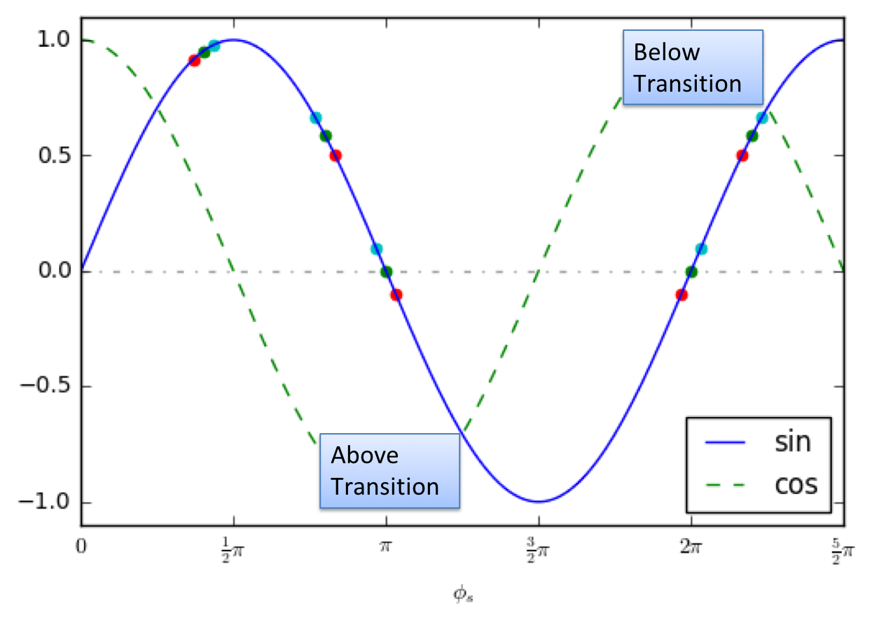
Summarizing the observations in the above example, we have the following table:
| Energies | $\phi_s < \pi/2$ (Blue lines) |
$\phi_s > \pi/2$ (Yellow lines) |
Phase Space Rotation |
transition |
|---|---|---|---|---|
| High Energy, ($\eta>0$) | Unstable | Stable | Clockwise | Above Transition |
| Low Energy, ($\eta<0$) | Stable | Unstable | Counter- Clockwise |
Below Transition |
Then Let's consider the case when the beam is accelerated by the RF cavity. The energy gain per turn is very small compare with the beam energy. In this case, the phase space variable should be properly used. In the following example, the area of phase space of $(\phi, \delta)$ does not conserve anymore. If the acceleration is slow the phase space of $(\phi, \Delta E)$ is nearly conserved. Here, we have to assume that:
\begin{align} \frac{2\pi h \eta}{\beta^2 E_0} \approx \text{constant} \end{align}turns=10000
sin_phi_s=0.5
beam_energy=100e9
mass=0.938e9
harm=360
voltage=5e6
update_eta=True
# Gamma and Betas
gamma=beam_energy/mass
mcf=0.04
eta=mcf-1/gamma/gamma
beta=np.sqrt(1-1/gamma/gamma)
# Calculate the bucket height
phi_s=np.arcsin(sin_phi_s)
yf=np.sqrt(np.cos(phi_s)-(np.pi-2*phi_s)*np.sin(phi_s)/2)
height=2*np.sqrt(voltage/2/np.pi/beta/beta/beam_energy/harm/np.abs(eta))*yf
#print(height)
phi_0=np.pi-phi_s
#phi_0=phi_s
delta_0=height*1.0*beam_energy
# Use phi-delta phase space
npar=1
initial_phi=np.ones(npar)*(phi_0)
initial_de=np.ones(npar)*delta_0
result=lde.longitudinal_evolve(turns,
initial_phi,
initial_de,
sin_phi_s=sin_phi_s, alphac=mcf, E0_ini=beam_energy,
mass=mass, e_volt=voltage, harm=harm,
update_eta=update_eta, energy_change=True
)
fig,(ax1,ax2)=plt.subplots(1,2, figsize=(10,5))
ax1.set_title(r"Longitudinal Phase Space $(\phi,\delta)$")
ax2.set_title(r"Longitudinal Phase Space $(\phi,\Delta E)$")
ax1.set_xlabel('Phase [rad]')
ax2.set_xlabel('Phase [rad]')
ax1.set_ylabel(r'$\delta=dp/p_0$')
ax2.set_ylabel(r'$\Delta E [GeV]$')
#ax1.set_xlim([-np.pi,np.pi])
ax1.set_ylim([-2*height,2*height])
ax2.set_ylim([-2*height*beam_energy/1e9,2*height*beam_energy/1e9])
#ax1.set_prop_cycle(plt.cycler('color', plt.cm.Oranges(np.linspace(0, 1, 8))))
ax1.plot(result[0], result[2], linestyle='None', marker='.', markersize=0.1)
#ax2.set_prop_cycle(plt.cycler('color', plt.cm.Blues(np.linspace(0, 1, 8))))
ax2.plot(result[0], result[1]/1e9, linestyle='None',marker='.', markersize=0.1)
for ax in (ax1,ax2):
ax.set_xticks([-np.pi, -0.5*np.pi, 0., .5*np.pi, np.pi, 1.5*np.pi, 2*np.pi])
ax.set_xticklabels([r"$-\pi$", r"$-\frac{1}{2}\pi$", "$0$", r"$\frac{1}{2}\pi$",
r"$\pi$", r"$\frac{3}{2}\pi$", r"$2\pi$"])
ax.set_xlim([-0,2*np.pi])
plt.tight_layout()

When the acceleration rate is fast, the $(\phi, \Delta E)$ is not a closed circle anymore. See the following example for medical therapy:
turns=300
sin_phi_s=0.5

mass=0.938e9
beam_energy=45e6+mass
p0=np.sqrt(beam_energy*beam_energy-mass*mass)
harm=1
voltage=0.1e6
mcf=0.05
update_eta=True
# Gamma and Betas
gamma=beam_energy/mass
eta=mcf-1/gamma/gamma
beta=np.sqrt(1-1/gamma/gamma)

# Calculate the bucket height
phi_s=np.arcsin(sin_phi_s)
yf=np.sqrt(np.cos(phi_s)-(np.pi-2*phi_s)*np.sin(phi_s)/2)
height=2*np.sqrt(voltage/2/np.pi/beta/beta/beam_energy/harm/np.abs(eta))*yf
#print(height)


phi_0=np.pi-phi_s
#phi_0=phi_s
delta_E=.3e6 ## MeV
delta_P=np.sqrt((beam_energy+delta_E)*(beam_energy+delta_E)-mass*mass)/p0-1
# Use phi-delta phase space
npar=2
initial_phi=np.ones(npar)*(phi_0)
initial_de=np.linspace(0,1, npar)*delta_E

result=lde.longitudinal_evolve(turns,
                                       initial_phi,
                                       initial_de,
                                       sin_phi_s=sin_phi_s, alphac=mcf, E0_ini=beam_energy,
                                       mass=mass, e_volt=voltage, harm=harm,
                                       update_eta=update_eta, energy_change=True
                                      )

fig,(ax1,ax2)=plt.subplots(1,2, figsize=(10,5))
ax1.set_title(r"Longitudinal Phase Space $(\phi,\delta)$")
ax2.set_title(r"Longitudinal Phase Space $(\phi,\Delta E)$")
ax1.set_xlabel('Phase [rad]')
ax2.set_xlabel('Phase [rad]')
ax1.set_ylabel(r'$\delta=dp/p_0$')
ax2.set_ylabel(r'$\Delta E [MeV]$')
#ax1.set_xlim([-np.pi,np.pi])
ax1.set_ylim([-2*height,2*height])
ax2.set_ylim([-2*height*beam_energy*beta*beta/1e6,2*height*beta*beta*beam_energy/1e6])
#ax1.set_prop_cycle(plt.cycler('color', plt.cm.Oranges(np.linspace(0, 1, 8))))
ax1.plot(result[0], result[2], linestyle=None)
#ax2.set_prop_cycle(plt.cycler('color', plt.cm.Blues(np.linspace(0, 1, 8))))
ax2.plot(result[0], result[1]/1e6, linestyle=None)

for ax in (ax1,ax2):
    ax.set_xticks([-np.pi, -0.5*np.pi, 0., .5*np.pi, np.pi, 1.5*np.pi, 2*np.pi])
    ax.set_xticklabels([r"$-\pi$", r"$-\frac{1}{2}\pi$", "$0$", r"$\frac{1}{2}\pi$",
                     r"$\pi$", r"$\frac{3}{2}\pi$", r"$2\pi$"])
    ax.set_xlim([-np.pi,2*np.pi])
plt.tight_layout()

Hamiltonian of longitudinal motion
The energy change is discrete. Over many turns, we approximate the change of the energy and phase is continuous. From
\begin{align} \delta_{n+1}&=\delta_{n} + \frac{eV}{\beta^2 E_0} \left(\sin \phi_n-\sin \phi_s\right)\\ \phi_{n+1}&=\phi_{n} + 2\pi h \eta \delta_{n+1} \end{align}We convert them to differential equations as:
\begin{align} \dot\delta&=\frac{eV\omega_0}{2\pi\beta^2E_0}\left(\sin\phi-\sin\phi_s\right) \label{eq:longi_H_eq_1} \\ \dot\phi&=h\omega_0\eta\delta \label{eq:longi_H_eq_2} \end{align}where $\omega_0$ is the revolution frequency. Combine the two equations, we get the second order differential equation:
\begin{align} \ddot\phi=\frac{eVh\eta\omega_0^2}{2\pi\beta^2E_0}\left(\sin\phi-\sin\phi_s\right) \end{align}fig,ax=plt.subplots()
ax.set_xlabel('Phase [rad]')
ax.set_ylabel('Potential [Arb. unit]')
phi=np.linspace(-np.pi,4*np.pi,100)
phi_s=np.pi/6
ax.plot(phi, (np.cos(phi)-np.cos(phi_s)+np.sin(phi_s)*(phi-phi_s)), label=r'$\eta<0$; $\phi_{stable}=5\pi/6$')
phi_s=0
ax.plot(phi, (np.cos(phi)-np.cos(phi_s)+np.sin(phi_s)*(phi-phi_s)), label=r'$\eta<0$; $\phi_{stable}=\pi$')
ax.axhline(y=0, ls='--', c='g')
ax.set_xticks([-np.pi, -0.5*np.pi, 0., .5*np.pi, np.pi, 1.5*np.pi, 2*np.pi])
ax.set_xticklabels([r"$-\pi$", r"$-\frac{1}{2}\pi$", "$0$", r"$\frac{1}{2}\pi$",
r"$\pi$", r"$\frac{3}{2}\pi$", r"$2\pi$"])
ax.legend(loc='best')

If we construct a longitudinal Hamiltonian as below, the above differential equation is the same form as the Hamiltonian equation:
\begin{equation} H(\phi,\delta)=\frac{1}{2}h\omega_0\eta\delta^2+\frac{eV\omega_0}{2\pi\beta^2E_0}\left[\cos\phi-\cos\phi_s+\sin\phi_s\left(\phi-\phi_s\right)\right] \end{equation}Above plots shows the phase dependence and the stable region.
Small amplitude approximation
At small phase deviation from $\phi_s$, $\Delta\phi=\phi-\phi_s$, we have
\begin{equation} \ddot{\Delta\phi}=\frac{eVh\eta\omega_0^2}{2\pi\beta^2E_0}\cos\phi_s \Delta\phi \end{equation}To have a stable motion, we require that:
\begin{equation} \eta\cos\phi_s <0 \end{equation}Under the stable condition, the small amplitude synchrotron tune is defined as:
\begin{equation} Q_s=\sqrt{\frac{-eVh\eta\cos\phi_s}{2\pi\beta^2E_0}}\equiv\nu_s\sqrt{\left|\cos\phi_s\right|} \end{equation}Often, the $\nu_s$ is referred as synchrotron tune with $\phi_s=n\pi$.
And we can write the small amplitude Hamiltonian as:
\begin{equation} H=\frac{1}{2}h\omega_0\eta\delta^2+\frac{eV\omega_0\left(-\cos\phi_s\right)}{4\pi\beta^2E_0}\Delta\phi^2 \end{equation}For fixed energy of the Hamiltonian, we can get the phase space shape, which is sets of ellipse.
\begin{equation} \left(\frac{\delta}{\left<\delta\right>}\right)^2+\left(\frac{\Delta\phi}{\left<\Delta\phi\right>}\right)^2=1 \end{equation}with:
\begin{align} \left<\delta\right>&=\mathcal{A}\sqrt{\frac{2}{h\omega_0\eta}}\\ \left<\Delta\phi\right>&=\mathcal{A}\sqrt{\frac{4\pi\beta^2E_0}{eV\omega_0\left(-\cos\phi_s\right)}}\\ \end{align}The ratio gives:
\begin{equation} \frac{\left<\delta\right>}{\left<\Delta\phi\right>}=\sqrt\frac{eV\left(-\cos\phi_s\right)}{2\pi h\eta\beta^2E_0}=\frac{Q_s}{h\left|\eta\right|} \end{equation}It is interesting to check the flow of the phase space trajectory. For $\eta > 0$, we have a positive 'mass' system, the phase space flow is clockwise, while for the $\eta < 0$, the Hamiltonian become negative, and the phase space flow is counter-clockwise.
Unstable fix point and bucket
Through the behavior of the unstable fix point, we can define a separatrix that separate the stable and non-stable region. Suppose we have pair of $\eta$ and $\phi_s$ to have a stable motion. the phase space point $(\pi-\phi_s, 0)$ will be the unstable point with the 'energy':
\begin{equation} E_{sep}=H(\pi-\phi_s,0)=\frac{eV\omega_0}{2\pi\beta^2E_0}\left[-2\cos\phi_s+\sin\phi_s\left(\pi-2\phi_s\right)\right] \end{equation}Then the separatrix is defined by:
\begin{equation} H(\phi,\delta)=E_{sep} \end{equation}\begin{equation} \frac{1}{2}h\omega_0\eta\delta_{sp}^2+\frac{eV\omega_0}{2\pi\beta^2E_0}\left[\cos\phi+\cos\phi_s-\sin\phi_s\left(\pi-\phi-\phi_s\right)\right]=0 \end{equation}The separatrix explicitly expressed as:
\begin{equation} \delta_{sp}=\sqrt{\frac{eV}{\pi\beta^2 E_0 h\eta}\left[-\cos\phi-\cos\phi_s+\sin\phi_s\left(\pi-\phi-\phi_s\right)\right]} \end{equation}The turning point $\phi_u$ is the point where $\delta=0$:
\begin{equation} -\cos\phi_u-\cos\phi_s+\sin\phi_s\left(\pi-\phi_u-\phi_s\right)=0 \end{equation}or
\begin{equation} \cos\phi_u+\phi_u\sin\phi_s=-\cos\phi_s+\sin\phi_s\left(\pi-\phi_s\right) \end{equation}The maximum height is
\begin{align} \delta_{max}(\phi_s)&=\delta_{sp}(\phi_s) \nonumber\\ &=\sqrt{\frac{eV}{\pi\beta^2 E_0 h\eta}\left[-2\cos\phi_s+\sin\phi_s\left(\pi-2\phi_s\right)\right]} \\ &=\delta_{max}(\phi_s=0)\sqrt{\left|-\cos\phi_s+\sin\phi_s\left(\pi-2\phi_s\right)/2\right|} \end{align}The bucket area reads:
\begin{align} \mathcal{A_b} &= 2\int_{\phi_u}^{\pi-\phi_s}\delta_{sp}(\phi)d\phi \nonumber\\ &=2\sqrt{\frac{2eV}{\pi\beta^2 E_0 h\left|\eta\right|}} \int_{\phi_u}^{\pi-\phi_s}\frac{1}{\sqrt{2}}\left|\cos\phi+\cos\phi_s-\sin\phi_s\left(\pi-\phi-\phi_s\right)\right|^{1/2} d\phi\\ &\equiv \mathcal{A_b} (\phi_s=0) \int_{\phi_u}^{\pi-\phi_s}\frac{1}{4\sqrt{2}}\left|\cos\phi+\cos\phi_s-\sin\phi_s\left(\pi-\phi-\phi_s\right)\right|^{1/2} d\phi \end{align}# Bucket shape for eta < 0
import scipy.optimize as opt
#phi_s=np.pi/3
def fangle(phi, phis):
return (np.cos(phi)+np.cos(phis)-np.sin(phis)*(np.pi-phi-phis))/2.0
def gen_plot_data(phis):
phi_u=opt.fsolve(fangle, (phis-np.pi)/3.0, args=(phis,))
extra=(np.pi-phis-phi_u)/3.0
phi_list=np.linspace(phi_u, np.pi-phis+extra,300)
delta_list=np.sqrt(np.abs(fangle(phi_list, phis)))
return np.concatenate([ np.flip(phi_list,0), phi_list]),np.concatenate([np.flip(delta_list,0), -delta_list])
fig,ax=plt.subplots()
ax.set_xlabel("Phase [rad]")
ax.set_ylabel(r"$\delta_{max}/\delta_{max}(\phi_s=0)$")
temp=gen_plot_data(1e-8)
ax.plot(temp[0],temp[1], label=r"$\phi_s=0$")
temp=gen_plot_data(np.pi/6)
ax.plot(temp[0],temp[1], label=r"$\phi_s=\pi/6$")
temp=gen_plot_data(np.pi/4)
ax.plot(temp[0],temp[1], label=r"$\phi_s=\pi/4$")
temp=gen_plot_data(np.pi/3)
ax.plot(temp[0],temp[1], label=r"$\phi_s=\pi/3$")
#ax.plot(phi_list,-delta_list, c='b')
ax.set_xticks([-np.pi, -0.5*np.pi, 0., .5*np.pi, np.pi, 1.5*np.pi, 2*np.pi])
ax.set_xticklabels([r"$-\pi$", r"$-\frac{1}{2}\pi$", "$0$", r"$\frac{1}{2}\pi$",
r"$\pi$", r"$\frac{3}{2}\pi$", r"$2\pi$"])
ax.legend(loc='best')

from scipy import integrate
def sqrt_fangle(phi,phis):
    return np.sqrt(fangle(phi,phis))
def bucket_area(phis):
    phi_u=opt.fsolve(fangle, (phis-np.pi)/3.0, args=(phis,))
    return integrate.quad(sqrt_fangle, phi_u, np.pi-phis, args=(phis,))[0]
phis_list=np.linspace(0, np.pi/2, 300, endpoint=False)[1:]
area=[]
for phis in phis_list:
    area.append(bucket_area(phis)/4)
fig,ax=plt.subplots()
ax.set_xlim([0,np.pi/2.0])
ax.set_ylabel(r"Relative Bucket area")
ax.set_xlabel(r"Synchronous phase [rad]")
ax.set_xticks(np.linspace(0,0.5,5,)*np.pi)
ax.set_xticklabels(["$0$", r"$\frac{1}{8}\pi$", r"$\frac{1}{4}\pi$",
                    r"$\frac{3}{8}\pi$", r"$\frac{1}{2}\pi$",
                     ])

ax.plot(phis_list, area)

The action of the synchrotron motion is defined from the Hamiltonian with fixed 'energy':
\begin{align} H(\phi,\delta)=\frac{1}{2}h\omega_0\eta\delta^2+\frac{eV\omega_0}{2\pi\beta^2E_0}\left[\cos\phi-\cos\phi_s+\sin\phi_s\left(\phi-\phi_s\right)\right]=H_0 \end{align}The action $J$ is calculated by:
\begin{align} J&=\frac{1}{2\pi}\oint \delta d\phi\\ &=\frac{1}{2\pi} \sqrt{\frac{2}{h\omega_0\eta}}\oint \left(H_0-\frac{eV\omega_0}{2\pi\beta^2E_0}\left(\cos\phi-\cos\phi_s+\sin\phi_s\left(\phi-\phi_s\right)\right)\right)^{\frac{1}{2}}d\phi \end{align}Therefore the period of the motion can be calculated as
\begin{align} T&=\frac{2\pi}{\omega}=2\pi\left(\frac{dJ}{dH_0}\right) \\ &=\sqrt{\frac{1}{2h\omega_0\eta}}\oint \left(H_0-\frac{eV\omega_0}{2\pi\beta^2E_0}\left(\cos\phi-\cos\phi_s+\sin\phi_s\left(\phi-\phi_s\right)\right)\right)^{-\frac{1}{2}}d\phi \end{align}When the synchronous phase satisfy $\sin\phi_s=0$, viz that $\phi_s=0$ or $\phi_s=\pi$, we can compare the longitudinal Hamiltonian with the Hamiltonian of a pendulum system:
| Longitudinal Motion | Items | Pendulum Motion |
|---|---|---|
| $H=\frac{1}{2}h\omega_0\eta\delta^2+\frac{eV\omega_0}{2\pi\beta^2E_0}\left(\cos\phi\pm 1\right)$ | Hamiltonian | $H=\frac{1}{2}m v^2+mgl\left(1-\cos\phi\right)$ |
| $h\omega_0\eta$ | 'Mass' | $m$ |
| $0(\eta<0)$ or $\pi(\eta>0)$ | Stable phase |
0 |
| $\pm\sqrt{\frac{2eV}{\pi\beta^2E_0h\eta}}$ | Bucket height |
$2\sqrt{gl}$ |
| $\omega_0\sqrt{\frac{-eVh\eta\cos\phi_s}{2\pi\beta^2E_0}}$ | $\omega$ of Small amplitude |
$\sqrt{g/l}$ |
Longitudinal phase space area
The longitudinal phase space area can be defined have similar definition as the transverse one. The most common variable pair is $(\Delta t, \Delta E)$. The advantage of such choice is that the phase space area does not change when cavities with multiple frequencies presents or acceleration is involved.
\begin{align} \mathcal{A}_{rms}=\pi\sqrt{\left<\Delta E\right>^2\left<\Delta t\right>^2-\left(\overline{\Delta E \Delta t}\right)^2} \end{align}We will see that the decoherence of due to the mismatch and de-coherence will quickly remove the correlation of the phase space therefore
\begin{align} \mathcal{A}_{rms}&\approx\pi\left<\Delta E\right>\left<\Delta t\right>\\ \mathcal{A}_{95\%}&\sim 6\mathcal{A}_{rms} \end{align}The unit of the phase area usually is eV-s.
%%HTML
<video width="320" height="240" controls>
  <source src="match.mp4" type="video/mp4">
</video>
<video width="320" height="240" controls>
  <source src="inj_error.mp4" type="video/mp4">
</video>
<video width="320" height="240" controls>
  <source src="slim_big.mp4" type="video/mp4">
</video>
<video width="320" height="240" controls>
  <source src="slim_small.mp4" type="video/mp4">
</video>
Near Transition Energy
If the transition energy is reached during the acceleration process of synchrotron, the dynamics at the vicinity of transition energy can be detailed. Suppose the acceleration rate is $\dot{\gamma}$ and passing the transition energy $\gamma_T$ at $t=0$, so that $\gamma(t)=\gamma_T+\dot{\gamma}t$. So the phase slip factor is
\begin{align} \eta(t)&=\alpha_c-\frac{1}{\gamma^2(t)}\\ &=\alpha_c-\frac{1}{\gamma_T^2}\left(1-\frac{2\dot\gamma t}{\gamma_T}+\mathcal{O}\left(\left(\frac{\dot\gamma t}{\gamma_T}\right)^2\right)\right)\\ &\approx \frac{2\dot\gamma t}{\gamma_T^3} \end{align}Here the time range is required to have $t \ll \gamma_T/\dot{\dot{\gamma}}$.
Recall that the synchrotron tune for small amplitude oscillation is:
\begin{equation} Q_s=\frac{\omega_s}{\omega_0}=\sqrt{\frac{-eVh\eta\cos\phi_s}{2\pi\beta^2E_0}} \end{equation}Near transision, the relation beomes:
\begin{equation}\label{eq:transition_freq} Q_s^2=\frac{\omega_s^2}{\omega_0^2}=\frac{-eVh \dot\gamma t \cos\phi_s}{\pi\gamma_T^4\beta^2 m c^2}\equiv \frac{1}{\omega_0^2 \tau_{ad}^3} t \end{equation}where $\tau_{ad}$ is parameter defined to charecterize the time that the tune change due to acceleration. We can check if the synchrotron tune $Q_s$ or frequency $\omega_s$ is change adiabatically, i.e. $\frac{1}{2\pi}\left|dT_s/dt\right| \ll 1$ where $T_s=2\pi/\omega_s$. Therefore the adabatic condition reads: $$ \frac{1}{\omega_s^2}\left|\frac{d\omega_s}{dt}\right| \ll 1 $$
with Eq.$\ref{eq:transition_freq}$, it becomes
$$ 4 \frac{\left|t\right|^3}{\tau_{ad}^3} \gg 1 $$or $$ \left|t\right| \gg 0.25^{1/3}\tau_{ad} $$ we can consider the system is adiabatic. The typical $\tau_{ad}$ value is milliseconds.
Under the small angle approximation, The Hamiltonian equation $\ref{eq:longi_H_eq_1}$ and $\ref{eq:longi_H_eq_2}$ near transition energy become:
\begin{align} \dot\delta&=\frac{eV\omega_0}{2\pi\beta^2E_0}\cos\phi_s \Delta \phi \label{eq:longi_H_eq_tran_eng_1} \\ \dot{\Delta\phi}&=\frac{2h\omega_0\dot\gamma t}{\gamma_T^3}\delta \label{eq:longi_H_eq_tran_eng_2} \end{align}Then, the second order ODE for $\delta$ and $\Delta\phi$ can be written as:
\begin{align} &\ddot\delta+\frac{t}{\tau_{ad}^3}\delta =0\\ &\frac{d}{dt}\left(\frac{\tau_{ad}^3}{t}\frac{d\Delta\phi}{dt}\right)+\Delta\phi=0 \end{align}The solution of equation for $\delta$ is Airy functions, while the solution of $\Delta\phi$ is Bessel function.
import sympy as sym
sym.init_printing()
tau=sym.symbols(r'\tau', real=True)
t = sym.symbols('t', real=True)
delta, phi = sym.symbols(r'\delta \phi', cls=sym.Function)
sym.dsolve(delta(t).diff(t,t)+t*delta(t)/tau**3, delta(t))
sym.dsolve((tau**3*phi(t).diff(t)/t).diff(t)+phi(t),phi(t))
from scipy.special import airy, jv, yv
tlist=np.linspace(0.001,1, 200)
ai, _, bi, _= airy(tlist)
be1= jv(2.0/3, 2.0*np.power(tlist,1.5)/3)
yn1= yv(2.0/3, 2.0*np.power(tlist,1.5)/3)
fig,ax=plt.subplots()
ax.plot(tlist,ai, label="Ai (t)")
ax.plot(tlist,bi, label="Bi (t)")
ax.set_ylim([0,1.5])
ax.legend(loc='best')

Connection to Linac Accelerator
Let's assume a standing-wave linac, which consists of a series of short accelerating gaps. Between the gap $n-1$ and $n$, the drift space has length $l_{n-1}$. The velocity of the ideal velocity in the drift space is $\beta_{n-1}$ and energy is $E_{n-1}$. The arriving time of ideal particle at gap $n$ is $t_{n}$ and phase is $\phi_{n}$. We use subscript $s$ to denote the reference particle.
The energy change is simply:
\begin{align} \Delta E_n=E_{n}-E_{s,n}&=\Delta E_{n-1}+eV\left(\sin\left(\phi_{s,n}+\Delta\phi_n\right)-\sin\phi_{s,n}\right) \\ &\approx \Delta E_{n-1}+eV \cos(\phi_{s,n})\Delta\phi_n \end{align}And the change of phase is simply:
\begin{align} \Delta \phi_n=\omega_0\left(t_{n}-t_{s,n}\right)&=\Delta \phi_{n-1}+\frac{\omega}{c}\left(\frac{l_{n-1}}{\beta_{n-1}}-\frac{l_{n-1}}{\beta_{s,n-1}}\right) \\ &\approx \Delta \phi_{n-1}-\frac{\omega}{c} \frac{l_{n-1}}{\beta_{s,n-1}^2}\Delta \beta_{n-1} \\ &=\Delta \phi_{n-1}-\frac{\omega}{mc^3} \frac{l_{n-1}}{\beta_{s,n-1}^3 \gamma_{s,n-1}^3}\Delta E_{n-1} \end{align}This map can be used to track the dynamics of linac. It is worthwhile to note that, since the momentum compaction factor of a linac is always zero ($\alpha_c=0$), the slip factor is always below zero ($\eta<0$), viz below transition.
If the acceleration rate is low and the gap between the acceleration gap is short, we may approximate the map using differential equation:
\begin{align} \frac{d\Delta E}{ds}&=e\mathcal{E}\left(\sin\left(\phi_{s}+\Delta\phi\right)-\sin\phi_{s}\right) \\ \frac{d\Delta \phi}{ds}&=-\frac{\omega}{mc^3\beta_{s}^3 \gamma_{s}^3}\Delta E \end{align}Here, $\mathcal{E}$ is the gradient of acceleration. Therefore the dynamics of linac and ring are very similar in this assumption, by just replacing the slip factor $\eta$ to $\frac{-1}{\gamma_s^2}$.
For small amplitude approximation, we have:
\begin{align} \frac{d^2\Delta E}{ds^2}&= -\frac{ e\mathcal{E}\omega\cos\phi_{s}}{mc^3\beta_{s}^3 \gamma_{s}^3}\Delta E \end{align}with the synchrotron oscillation wave number as:
\begin{align} k_s^{2}= \frac{ e\mathcal{E}\omega\cos\phi_{s}}{mc^3\beta_{s}^3 \gamma_{s}^3} \end{align}