Off Momentum Orbit

So far, we discussed the transverse dynamics for the particles with reference energy, or $$\delta = \frac{\Delta p}{p_0}=0$$

In this section, we will explore the transverse orbit properties for those particles with small momentum deviation $\delta$

Revisit the Hamiltonian

Let us recall the exact Hamiltonian has the form: $$K\left(x, p_x, y, p_y, z, \delta,s\right)=-\left(1+\frac{x}{\rho}\right)\sqrt{(1+\delta)^2-p_x^2-p_y^2} -e\frac{A_s}{p_0}\left(1+\frac{x}{\rho}\right) $$

With the paraxial approximation:

\begin{equation} K\left(x, p_x, y, p_y, z, \delta,s\right)= -\left(1+\frac{x}{\rho}\right)\left(1+\delta-\frac{p_x^2}{2(1+\delta)}-\frac{p_y^2}{2(1+\delta)}\right) -e\frac{A_s}{p_0}\left(1+\frac{x}{\rho}\right) \end{equation}

Keeping only up to the linear term of $delta$ and $x/\rho$, and using $$A_{s,d}\approx-B_0\left(x - \frac{x^2}{2\rho}\right)$$, $$A_{s,q}=-B_0 b_1(s) \left(x^2-y^2\right)/2=-G(s)\left(x^2-y^2\right)/2$$, we get:

\begin{align} K\left(x, p_x, y, p_y, z, \delta,s\right)&= -\left(1+\frac{x}{\rho}\right)\left(1+\delta-\frac{p_x^2}{2(1+\delta)}-\frac{p_y^2}{2(1+\delta)}\right) -e\frac{A_s}{p_0}\left(1+\frac{x}{\rho}\right)\\ &\approx -1-\delta-\delta\frac{x}{\rho}+\frac{p_x^2}{2}+\frac{p_y^2}{2}+\frac{x^2}{2\rho^2}+k(s)\left(x^2-y^2\right)/2 \end{align}

Here we assume $z$ and $\delta$ are parameter, therefore constants. The motion of $x$ any $y$ directions are still decoupled, and the Hamiltonian for the x direction is : $$ K\left(x, p_x\right)=\frac{p_x^2}{2}+\frac{x^2}{2\rho^2}+\frac{k(s)x^2}{2}-\delta\frac{x}{\rho} $$

Dispertion Function

The equation of motion then becomes a non-homogeneous one :

\begin{equation} x''+\left(\frac{1}{\rho^2}+k(s)\right)x=\frac{\delta}{\rho} \end{equation}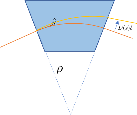

Clearly, the off-momentum orbit raises from the momentum deviation in the bending elements. If we write the solution as: $$ x(s)=x_\beta(s)+D(s)\delta + \mathcal{O}\left(\delta^2\right) $$

where $x_\beta(s)$ satisfies the homogeneous Hill's equation:

\begin{equation} x''+\left(\frac{1}{\rho^2}+k(s)\right)x=0 \end{equation}

The coefficient $D(s)=\frac{\partial x(s)}{\partial \delta}|_{\delta=0}$ is the linear dispersion function, which is also depend on the design lattice. It is the solution of the inhomogeneous ODE:

\begin{equation} D''+\left(\frac{1}{\rho^2}+k(s)\right)D=\frac{1}{\rho} \end{equation}

The solution of the dispersion function is the sum of the general solution of the homoneneous ODE and the special solution:

\begin{equation} \left(\begin{array}{c} D\\ D' \end{array}\right)_{s=s_{0}+s}=M\left(s_{0}+s,s_{0}\right)\left(\begin{array}{c} D\\ D' \end{array}\right)_{s=s_{0}}+\left(\begin{array}{c} d\\ d' \end{array}\right) \end{equation}

For constant dipole with fixed gradient, let's write $K=k+1/\rho^2$, the transver matrix $M$ has been calculated before:

\begin{equation} M\left(s_0+s,s_0\right)= \begin{cases} \left(\begin{array}{cc} \cos\left(\sqrt{K}s\right) & \sin\left(\sqrt{K}s\right)/\sqrt{K}\\ -\sqrt{K}\sin\left(\sqrt{K}s\right) & \cos\left(\sqrt{K}s\right) \end{array}\right)&K>0,\\ \\ \left(\begin{array}{cc} \cosh\left(\sqrt{K}s\right) & \sinh\left(\sqrt{K}s\right)/\sqrt{K}\\ \sqrt{K}\sinh\left(\sqrt{K}s\right) & \cosh\left(\sqrt{K}s\right) \end{array}\right)&K<0\\ \end{cases} \end{equation}

The spectial solution in this case, should satisfy $d(s=s_0)=d'(s=s_0)=0$, one can easily prove that the following expression satisfy the inhomogeous equation:

\begin{equation} d(s)= \begin{cases} \frac{1}{\rho K}\left( 1-\cos \left(\sqrt{K}s\right) \right)&K>0,\\ \frac{1}{\rho K}\left( 1-\cosh \left(\sqrt{-K}s\right) \right)&K<0 \end{cases} \end{equation}

and

\begin{equation} d'(s)= \begin{cases} \frac{1}{\rho \sqrt{K}} \sin \left(\sqrt{K} s \right) &K>0,\\ \frac{1}{\rho \sqrt{-K}} \sinh \left(\sqrt{-K}s \right)&K<0 \end{cases} \end{equation}

For pure dipole $K=1/\rho^2$, the special solution simply becomes:

\begin{align} d(s)&= \rho \left(1-\cos\theta\right) \approx\rho\theta^2\\ d'(s)&= \sin\theta \approx\theta \end{align}

Here $\theta=s/\rho$ is the bending angle. The approximation is taken when the bending angle for the dipole is small.

We can rewrite the matrix form in to a 3 by 3 matrix $\mathcal{M}$ and 3- vector form:

\begin{equation} \left(\begin{array}{c} D\\ D'\\ 1 \end{array}\right)_{s=s_{0}+s}=\left(\begin{array}{cc} {M}\left(s_{0}+s,s_{0}\right) & \bar{d}=\left(\begin{array}{c} d\\ d' \end{array}\right)\\ 0 & 1 \end{array}\right)\left(\begin{array}{c} D\\ D'\\ 1 \end{array}\right)_{s=s_{0}} \end{equation}

For pure dipole, we have the form:

\begin{align} \mathcal{M}_{dipole}&= \left(\begin{array}{ccc} \cos(\theta) & \rho\sin(\theta) & \rho\left(1-\cos\theta\right)\\ -\sin(\theta)/\rho & \cos(\theta) & \sin\theta\\ 0 & 0 & 1 \end{array}\right)\\ &\approx \left(\begin{array}{ccc} 1 & l & l\theta/2\\ 0 & 1 & \theta\\ 0 & 0 & 1 \end{array}\right)\\ \end{align}

Here, the approximation is again assuming short dipole and $l=\rho\theta$ is the length of the dipole.

Disperion with Periodic Condition

For a periodic lattice with length L, we must have the dispersion function satisfy $$ D\left(s_0\right)=D\left(s_0+L\right) \;;\; D'\left(s_0\right)=D'\left(s_0+L\right) $$

And the expanded $3\times3$ oneturn matrix has:

\begin{equation} \left(\begin{array}{c} D\\ D'\\ 1 \end{array}\right)_{s=s_0}=\left(\begin{array}{cc} M\left(s_{0}\right) & \left(\begin{array}{c} M_{13}\\ M_{23} \end{array}\right)\\ 0 & 1 \end{array}\right)\left(\begin{array}{c} D\\ D'\\ 1 \end{array}\right)_{s=s_{0}} \end{equation}

Here the matrix $M\left(s_0\right)$ is the oneturn betatron matrix:

\begin{align} M\left(s_0\right)&= \left(\begin{array}{cc} M_{11} & M_{12}\\ M_{21} & M_{22} \end{array}\right)\\ &=\left(\begin{array}{cc} \cos\Phi+\alpha\sin\Phi & \beta\sin\Phi\\ -\gamma\sin\Phi & \cos\Phi-\alpha\sin\Phi \end{array}\right) \end{align}

The elements $M_{13}$ and $M_{23}$ are related to the dispersion function by:

\begin{equation} \left(\begin{array}{c} M_{13}\\ M_{23} \end{array}\right)=\left(I-\left(\begin{array}{cc} M_{11} & M_{12}\\ M_{21} & M_{22} \end{array}\right)\right)\left(\begin{array}{c} D\\ D' \end{array}\right)\label{eq:matrix_from_dispersion} \end{equation}

The matrix $I-M\left(s_0\right)$ has determinant $2-M_{11}-M_{22}$ Recall that the stable condition of the periodic transfer matrix: $\left|Tr(M\left(s_0\right))\right|<2$, the determinant of $I-M\left(s_0\right)$ is always positive. Therefore we can reverse the Eq.$\ref{eq:matrix_from_dispersion}$ and calculate the dispersion function from the expanded one-turn matrix:

\begin{align} \left(\begin{array}{c} D\\ D' \end{array}\right) &=\left(I-M\right)^{-1}\left(\begin{array}{c} M_{13}\\ M_{23} \end{array}\right)\\ &=\frac{1}{2-M_{11}-M_{22}}\left(\begin{array}{cc} 1-M_{22} & M_{12}\\ M_{21} & 1-M_{11} \end{array}\right)\left(\begin{array}{c} M_{13}\\ M_{23} \end{array}\right)\label{eq:dispersion_from_matrix} \end{align}

$\mathcal{H}$ function

Since the dispersion function follows the inhomogeneous Hill's function, we can follow the action-angle treatment of the particle motion and define the normalized dispersion as:

\begin{align} X_d&=\frac{D}{\sqrt{\beta}}\\ P_d&=\frac{\beta D'+\alpha D }{\sqrt{\beta}} \end{align}

We define $\mathcal{H}$ function as

\begin{align} \mathcal{H}&\equiv X_d^2+P_d^2\\ &=\beta D'^2+2\alpha D D' + \gamma D^2 \end{align}

At the region outside dipole, $1/\rho=0$, the $\mathcal{H}$ function is constant. However, the bending field will change the value of the $\mathcal{H}$ function.

Dispersion measurement

The measurement of the dispersion in accelerator follows it definition:

\begin{equation} D=\frac{\partial x}{\partial \delta} \end{equation}

In a linac, this is straight forward to realize in real machine. One can easily change the energy of the beam by tweaking the accelerating cavity, then the dispersion is calculated from the beam centroid change at each Beam position monitor:

\begin{equation} D=\frac{\Delta x}{\Delta p/p_0} \end{equation}

The measurement in a ring will be not as trivial, since the change of the accelerating voltage will not affect the energy of the particle linearly. The dispersion measurement in a ring will be introduce in the later part of this note.

Integration Representation

From the similarity of the Hill's equation with dipole error and the dispersion equation:

\begin{equation} D''+\left(\frac{1}{\rho^2}+k(s)\right)D=\frac{1}{\rho} \end{equation}

and

\begin{equation} x''\left(s\right)+\left(\frac{1}{\rho^2}+k(s)\right)x\left(s\right)=\frac{\Delta B(s)}{B_0\rho} \end{equation}

The integrated form of dispersion function can be achieved from the closed orbit integrals by substituting $\frac{\Delta B(s)}{B_0\rho} $ with $\frac{1}{\rho}$.

\begin{align} D(s)&=\int_{s}^{s+C}\frac{1}{\rho(s_0)}G\left(s,s_{0}\right) ds_0 \nonumber\\ &=\frac{\sqrt{\beta\left(s\right)}}{{2\sin\pi\nu}} \int_{s}^{s+C}\frac{\sqrt{\beta\left(s_{0}\right)}}{\rho(s_0)}\cos\left(\psi\left(s\right)-\psi\left(s_{0}\right)-\pi\nu\right)ds_0 \end{align}

Dispersion Matching and Suppression

Achromatic Condition

For a lattice cell represented by $\mathcal{M}$, the acromatic condition guarantees that the if the zero dispersion is given at the entrance, zero dispersion is achieved at the exit.

\begin{equation} \left(\begin{array}{c} 0\\ 0\\ 1 \end{array}\right)=\left(\begin{array}{cc} {M}\left(s_{0}+s,s_{0}\right) & \bar{d}=\left(\begin{array}{c} M_{13}\\ M_{23} \end{array}\right)\\ 0 & 1 \end{array}\right)\left(\begin{array}{c} 0\\ 0\\ 1 \end{array}\right) \end{equation}

Therefore the acromatic condition requires:

\begin{equation} \bar{d}=\left(\begin{array}{c} M_{13}\\ M_{23} \end{array}\right) =\left(\begin{array}{c} 0\\ 0 \end{array}\right) \end{equation}

Dispersion Matching

Repeating cells

If we repeat a non-achromatic cell for N times, the $3\times 3$ matrix becomes:

\begin{align} \mathcal{M}^N&=\left(\begin{array}{cc} {M} & \bar{d}\\ 0 & 1 \end{array}\right)^N\\ &=\left(\begin{array}{cc} {M}^N & \left(M^{N-1}+M^{N-2}+\cdots+1\right)\bar{d}\\ 0 & 1 \end{array}\right)\\ &=\left(\begin{array}{cc} {M}^N & \left(I-M^{N} \right)\left(I-M \right)^{-1}\bar{d}\\ 0 & 1 \end{array}\right)\\ &=\left(\begin{array}{cc} {M}^N & \left(I-M^{N} \right)\left(\begin{array}{c} D\\ D' \end{array}\right)\\ 0 & 1 \end{array}\right) \end{align}

Therefore, to achieve a achromatic condition by repeating a non-achromatic cell $N$ times, it is required to have $$M^N=I$$

The betatron transfer matrix $M$ can be expressed by the twiss parameter:

\begin{equation} M=\left(\begin{array}{cc} \cos\Phi+\alpha\sin\Phi & \beta\sin\Phi\\ -\gamma\sin\Phi & \cos\Phi-\alpha\sin\Phi \end{array}\right) \end{equation}

Therefore the requirement becomes:

\begin{equation} N\Phi=2n\pi \;,\; n\in \text{Integer} \end{equation}

Dispersion suppression

For a non-achromatic lattice in a periodical structure, we have

\begin{equation} \left(\begin{array}{c} D\\ D'\\ 1 \end{array}\right)=\mathcal{M}\left(\begin{array}{c} D\\ D'\\ 1 \end{array}\right)= \left(\begin{array}{cc} M & \left(\begin{array}{c} M_{13}\\ M_{23} \end{array}\right)\\ 0 & 1 \end{array}\right)\left(\begin{array}{c} D\\ D'\\ 1 \end{array}\right) \end{equation}

A dispersion suppression section, represented by matrix $\tilde{\mathcal{M}}^{-1}$ can match a non-zero dispersion $(D,D')$ at the end of a curved lattice to zero dispersion, which reads

\begin{equation} \left(\begin{array}{c} D\\ D'\\ 1 \end{array}\right) = \tilde{\mathcal{M}} \left(\begin{array}{c} 0\\ 0\\ 1 \end{array}\right) = \left(\begin{array}{cc} \tilde{M} & \left(\begin{array}{c} \tilde{M}_{13}\\ \tilde{M}_{23} \end{array}\right)\\ 0 & 1 \end{array}\right)\left(\begin{array}{c} 0\\ 0\\ 1 \end{array}\right) \end{equation}

Then the required terms in the suppressor is simply:

\begin{equation} \left(\begin{array}{c} \tilde{M}_{13}\\ \tilde{M}_{23} \end{array}\right) = \left(\begin{array}{c} D\\ D' \end{array}\right) = \left(I-M\right)^{-1}\left(\begin{array}{c} M_{13}\\ M_{23} \end{array}\right) \end{equation}

We can use optimization methods to achieve such condition using any accelerator design software.

'Reduced-bending-field' suppressor

Generally, dispersion matching will change the optical functions as well. However, there are some special elegant case, which suppresses the dispersion while maintaining the optics. Suppose we have a lattice cell described by the transfer matrix $M$. It is non-achromatic and have:

\begin{equation} \left(\begin{array}{c} D\\ D'\\ 1 \end{array}\right)=\mathcal{M}\left(\begin{array}{c} D\\ D'\\ 1 \end{array}\right)= \left(\begin{array}{cc} M & \left(\begin{array}{c} M_{13}\\ M_{23} \end{array}\right)\\ 0 & 1 \end{array}\right)\left(\begin{array}{c} D\\ D'\\ 1 \end{array}\right) \end{equation}

and it satisfy $M^{2N}=I$. Therefore half of the $2N$ cell satisfy $M^N=-I$.

The $3\times 3$ matrix of the $N$ repeating cells is:

\begin{align} \mathcal{M}^N &=\left(\begin{array}{cc} M^N & \left(I-M^{N} \right)\left(I-M \right)^{-1}\left(\begin{array}{c} M_{13}\\ M_{23} \end{array}\right)\\ 0 & 1 \end{array}\right)\\ &=\left(\begin{array}{cc} -I& 2\left(\begin{array}{c} D\\ D' \end{array}\right)\\ 0 & 1 \end{array}\right) \end{align}

We know that the dispersion term is proportional to its bending angle, however, in small angle approximation, the betatron transverse matrix does not depend on the bending angle.

Therefore it is now easy to come up a scheme to suppress the dispersion from a non-achromatic cell to zero dispersion.

• Make the cell N times so that the transfer matrix for the N cells is $-I$
• Reduce all dipole bending angle to its half value.

Then after some small modification, we can get a lattice that suppress the dispersion yet keep the original optics function.

Momentum Compaction Factor

In a ring or an arc, it is important to knew the pass length of the particle. The ideal particle must have the desire trajectory length to synchronize with the RF cavity for acceleration. We also need to calculate the pass length difference for an off-momentum particle.

Generally, we can calculate the circumference as:

\begin{align} C&=\oint\left|\frac{d\mathbf{r}(s)}{ds}\right|ds\nonumber\\ &=\oint\left|\frac{d\left(\mathbf{r_{0}}(s)+x\hat{x}+y\hat{y}\right)}{ds}\right|ds\nonumber\\ &=\oint\left|(1+x/\rho)\hat{s}+x'\hat{x}+y'\hat{y}\right|ds\nonumber\\ &=\oint\sqrt{\left(1+x/\rho\right)^{2}+x'^{2}+y'^{2}}ds \end{align}

If we keep only the linear term, then plug in the off-momentum term, we have

\begin{align} C&=\oint\left(1+\frac{x}{\rho}\right) ds \nonumber\\ &=C_0+\oint\left(\frac{x_\beta+D\delta}{\rho}\right) ds \nonumber\\ &=C_\beta+\left(\oint\frac{D}{\rho} ds \right)\delta \end{align}

This indicates that the extra circumference of the off-momentum is proportional to the momentum deviation. We define the Momentum Compaction Factor as:

\begin{equation} \alpha_c=\frac{1}{C_0}\frac{dC}{d\delta}=\frac{1}{C_0}\oint\frac{D}{\rho}ds \end{equation}

Since the dispersion function is usually positive, the momentum compaction factor is also positive. This means the higher energy particles usually travels longer. However there are special lattice which is designed to have zero or even negative compaction factor.

We can also calculate the travel time $t=C/v$ difference of the off-momentum particles:

\begin{align} \frac{\Delta T}{T}&=\frac{\Delta C}{C}-\frac{\Delta v}{v}\\ &=\alpha_c \delta-\frac{1}{\gamma^2}\delta\\ &\equiv\eta \delta \end{align}

The new quantity $\eta=dT/d\delta$ is named phase-slip factor, which is very useful in the latter longitudinal dynamics. In suggests that, for a positive momentum compaction factor $\alpha_c$, viz. that higher energy particles travels longer, may spend less time if the reference energy is low enough. At specific energy, a small momentum deviation does not change the time-of-flight, which is called isochronous. This energy is called transition energy $\gamma_T$:

\begin{equation} \gamma_T\equiv\frac{1}{\sqrt{\alpha_c}} \end{equation}

Dispersion Measurement in Ring

In a ring, changing the RF cavity produce more complicate behavior than in a linac. We will introduce that in the longitudinal dynamics section. However, the change of the beam energy is linked with the time-of-flight and the revolution frequency by phase-slip factor.

\begin{equation} \frac{\Delta f}{f_0}=-\frac{\Delta T}{T_0}=-\eta \delta \end{equation}

Therefore, the dispersion can be found from the slope of the closed orbit as function of the revolution frequency:

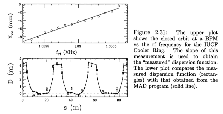
\begin{equation} D=\frac{\Delta x_{co}}{\delta}=-\eta f_0\frac{\Delta x_{co}}{\Delta f} \end{equation}

The following example (from "Accelerator Physics" by Prof. S.Y.Lee) shows the measurement data of IUCF cooler ring. The top figure is the closed orbit as function of the revolution frequency at one BPM. The bottom figure is the dispersion function at BPMs using the slope of the top figure of each BPM.

Transition Energy Crossing

In a medium energy synchrotron, there are many harmful beam dynamics problems when crossing the transition energy ($\gamma=\gamma_T$),viz the machine becomes isochronous. In this section, we briefly introduce the scheme to avoid the harmful effect.

$\gamma_T$ jump

One idea of avoiding the harmful effect of crossing transition energy is to cross the transition energy fast, using a set of pulsed power quadrupoles (named $\gamma_T$ quad). These quads, after turned on, can change the momentum compaction factor quick enough the decrease the $\gamma_T$ almost 'suddenly'.

These quads has to be placed in dispersive area, where the kick to the off-momentum particle by the ith quad is

\begin{equation} \Delta \theta_i= K_i \tilde{D}_i\delta \end{equation}

The quad will change the dispersion function over the ring and disturb the dispersion at the location from $D_i$ to $\tilde{D}_i$

Then the momentum compaction change will be:

\begin{equation} \Delta \alpha_c= \frac{\sum_i D_i \Delta \theta_i }{C_0\delta} =\frac{1}{C_0}\sum_i K_i \tilde{D}_i D_i \end{equation}

Flexible momentum compaction (FMC) lattice

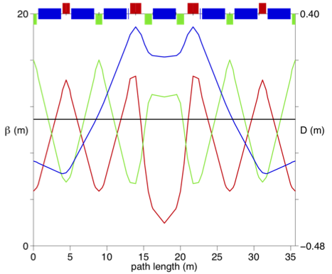
Another choice is to have zero or even negative momentum compaction factor $\alpha_c$. From the definition of $\alpha_c$, we have to design a lattice with negative dispersion at dipoles. That is turned out to be possible. One example is shown below, which is a cell for an ERL recently. The dispersion is design to have positive and negative numbers and the integrals in the

6-D phase space

The 3-by-3 matrix $\mathcal{M}$ describes the horizontal phase space as function of the energy. That is not a full description. The symplectic condition requires that if the horizontal phase space is affected by the longitudinal coordinate ($\delta$), the longitudinal phase space coordinate must be affected by the horizontal coordinates.

Therefore, the full dynamics has to be described by 6-by-6 matrix.

\begin{align} \left(\begin{array}{c} x\\ p_{x}\\ y\\ p_{y}\\ z\\ \delta \end{array}\right)_{2}=\left(\begin{array}{cccccc} R_{11} & R_{12} & R_{13} & R_{14} & R_{15} & R_{16}\\ R_{21} & R_{22} & R_{23} & R_{24} & R_{25} & R_{26}\\ R_{31} & R_{32} & R_{33} & R_{34} & R_{35} & R_{36}\\ R_{41} & R_{42} & R_{43} & R_{44} & R_{45} & R_{46}\\ R_{51} & R_{52} & R_{53} & R_{54} & R_{55} & R_{56}\\ R_{61} & R_{62} & R_{63} & R_{64} & R_{65} & R_{66} \end{array}\right)\left(\begin{array}{c} x\\ p_{x}\\ y\\ p_{y}\\ z\\ \delta \end{array}\right)_{1} \end{align}

The $R$ matrix represents the linear map for the 6-D phase space.
For lattice that only contains DC magnets and pure accelerating cavities, the arriving time does not affect the transverse phase space. As a consequence of symplecticity, the energy will not affected by the initial transverse phase phase space. Therefore:

\begin{align} R_{15}=R_{25}=R_{35}=R_{45}&=0\\ R_{61}=R_{62}=R_{63}=R_{64}&=0 \end{align}

When there is no accelerating components, $R_{65}$ is also zero. Also in the special case when there is no transverse coupling, the $R_{51}$ and $R_{52}$ is only related to $R_{16}$ and $R_{26}$ by:

\begin{align} R_{51}=(-R_{26})R_{11}+(R_{16})R_{21}\\ R_{52}=(-R_{26})R_{12}+(R_{16})R_{22}\\ \end{align}

or vector form:

\begin{align} \left(\begin{array}{cc} R_{51} & R_{52}\end{array}\right)=\left(\begin{array}{cc} -R_{26} & R_{16}\end{array}\right)\left(\begin{array}{cc} R_{11} & R_{12}\\ R_{21} & R_{22} \end{array}\right) \end{align}

Similarly we have for vertical direction:

\begin{align} \left(\begin{array}{cc} R_{53} & R_{54}\end{array}\right)=\left(\begin{array}{cc} -R_{36} & R_{46}\end{array}\right)\left(\begin{array}{cc} R_{33} & R_{34}\\ R_{43} & R_{44} \end{array}\right) \end{align}