Perturbation of transverse motion
The Hamiltonian of an unperturbed motion is
\begin{align} H=\frac{p_x^2}{2}+\frac{p_y^2}{2}+\left(\frac{1}{2\rho^2}+\frac{k(s)}{2} \right) x^2-\frac{k(s)}{2}y^2 \end{align}Now we assume that the motion is perturbed by $\Delta \mathbf{B}(s) = \Delta B_x(s) \hat{x}+\Delta B_y(s) \hat{y}$, where
\begin{align} \Delta B_y+i\Delta B_x &= B_0 \sum_{n=0}^\infty \left(\Delta b_n + i \Delta a_n\right) \left(x+iy\right)^{n} \end{align}The vector potential becomes:
\begin{align} \Delta A_s=-B_0 \Re \sum_{n=0}^\infty \frac {b_n + i a_n}{n+1} \left(x+iy\right)^{n+1} \end{align}The Hamiltonian becomes:
\begin{align} H=\frac{p_x^2}{2}+\frac{p_y^2}{2}+\left(\frac{1}{2\rho^2}+\frac{k(s)}{2} \right) x^2-\frac{k(s)}{2}y^2 \pm \frac{1}{B\rho} \Delta A_s \end{align}Here, the plus and minus sign reflect the negative and positive charge particle respectively.
Then the Hill's equation becomes:
\begin{align} x''+\left(\frac{1}{\rho^2}+k(s)\right)x&= -\frac{\Delta B_y}{B\rho} \\ y''-k(s)y&=\frac{\Delta B_x}{B\rho} \end{align}If $\Delta B_y$ is not a function of $y$, and $\Delta B_x$ is not a function of $x$, these two equation remain decoupled. The linear effect of uncoupled case will be introduce in the next two sub-sections. The linear coupled case will be introduced in the last sub-section.
Perturbed orbit
The perturbed orbit rises from the dipole errors, which can be contributed from a dipole strength error or a quadrupole misalignment.
Green function of Hill's equation
At the present of the dipole error, the general Hill's equation becomes:
\begin{equation} x''\left(s\right)+\kappa\left(s\right)x\left(s\right)=-\frac{\Delta B_y(s)}{B_0\rho} \end{equation}The solution can be retrieved from the Green's function method. The green function is the solution of:
\begin{equation} x''\left(s\right)+\kappa\left(s\right)x\left(s\right)=\theta\delta\left(s-s_0\right) \end{equation}This shows that a delta function dipole changes the orbit by $\theta$ at location $s_0$
Integrate the function at the vicinity of the $s_0$ gives:
\begin{equation} x'\left(s_{0+}\right)-x'\left(s_{0-}\right)=\theta \label{eq:angle_kick} \end{equation}Linac accelerator
From the linear accelerator, the beam only pass $s_0$ once. From the transfer matrix from $s_0$ to $s_1$
\begin{equation} M\left(s_{1}\mid s_{0}\right) =\left(\begin{array}{cc} \sqrt{{\frac{\beta_{1}}{\beta_{0}}}}\left(\cos\psi+\alpha_{0}\sin\psi\right) & \sqrt{\beta_{0}\beta_{1}}\sin\psi\\ -\frac{1+\alpha_{0}\alpha_{1}}{\sqrt{\beta_{0}\beta_{1}}}\sin\psi+\frac{\alpha_{0}-\alpha_{1}}{\sqrt{\beta_{0}\beta_{1}}}\cos\psi & \sqrt{{\frac{\beta_{0}}{\beta_{1}}}}\left(\cos\psi-\alpha_{1}\sin\psi\right) \end{array}\right) \label{eq:tmatrix_s0s1} \end{equation}where $\psi(s)=\psi(s_1)-\psi(s_0)$. We get the response of the delta dipole error, or the Green's function (normalized by $\theta$) as:
\begin{equation} G(s, s_0)=\frac{x(s)}{\theta}=\sqrt{\beta_{s}\beta_{s_0}}\sin\left(\psi\left(s\right)-\psi\left(s_0\right)\right) H\left(s-s_0\right) \end{equation}Here, $H(x)$ is the Heaviside step function.
Then for an arbitrary dipole error distribution $\frac{\Delta B(s)}{B_0\rho}$, the centroid orbit becomes:
\begin{align} x(s) &=\int_{-\infty}^{\infty}\frac{\Delta B(s_0)}{B_0\rho}G(s,s_0)ds_0 \nonumber\\ &=\sqrt{\beta(s)}\int_{-\infty}^{s}\frac{\sqrt{\beta(s_0)}\Delta B(s_0)}{B_0\rho}\sin\left(\psi\left(s\right)-\psi\left(s_0\right)\right) ds_0 \end{align}Ring accelerator
In ring accelerator, the beam will pass $s_0$ many times. There exist a stable orbit, deviate from the reference orbit, due to the dipole error. This is called closed orbit.
In every turn, the beam will have a kick at $s_0$ described in $\ref{eq:angle_kick}$. Combined with the one-turn matrix $M(s_0)$,
\begin{equation} M\left(s_{0}\right)= \left(\begin{array}{cc} \cos\Phi+\alpha_{0}\sin\Phi & \beta_{0}\sin\Phi\\ -\frac{1+\alpha_{0}^{2}}{\beta_{0}}\sin\Phi & \cos\Phi-\alpha_{0}\sin\Phi \end{array}\right) \end{equation}Here $\Phi=2\pi\nu$. we have a closed orbit condition:
\begin{equation} \left(\begin{array}{c} x\\ x'_{-}=x'_{+}-\theta \end{array}\right)= \left(\begin{array}{cc} \cos\Phi+\alpha_{0}\sin\Phi & \beta_{0}\sin\Phi\\ -\frac{1+\alpha_{0}^{2}}{\beta_{0}}\sin\Phi & \cos\Phi-\alpha_{0}\sin\Phi \end{array}\right) \left(\begin{array}{c} x\\ x'_{+} \end{array}\right) \end{equation}Solve the equation, we have:
\begin{equation} \left(I-M\right) \left(\begin{array}{c} x\\ x'_{+} \end{array}\right) = \left(\begin{array}{c} 0\\ \theta \end{array}\right) \end{equation}From the $\det(I-M)=2-2\cos\Phi$ the stable value of $x$ can be easily found as:
\begin{align} x(s_0)&=\frac{\beta\left(s_0\right)\sin\Phi}{2-2\cos\Phi}\theta=\frac{\beta\left(s_0\right)\cos\pi\nu}{2\sin\pi\nu}\theta \\ x'(s_{0+})&=\frac{1-\cos\Phi-\alpha\sin\Phi}{2-2\cos\Phi}\theta=\frac{\sin\pi\nu-\alpha\left(s_0\right)\cos\pi\nu}{2\sin\pi\nu}\theta \end{align}Here, the betatron tune is $\nu$. Then using the transfer matrix $\ref{eq:tmatrix_s0s1}$, we get the Green's function:
\begin{align} G\left(s,s_{0}\right) & =\frac{x(s)}{\theta}\nonumber\\ & =\frac{\sqrt{\beta\left(s\right)\beta\left(s_{0}\right)}}{{2\sin\pi\nu}}\left(\cos\pi\nu\left(\cos\psi+\alpha\left(s_{0}\right)\sin\psi\right)+\sin\psi\left(\sin\pi\nu-\alpha\left(s_{0}\right)\cos\pi\nu\right)\right)\nonumber\\ & =\frac{\sqrt{\beta\left(s\right)\beta\left(s_{0}\right)}}{{2\sin\pi\nu}}\cos\left(\psi\left(s\right)-\psi\left(s_{0}\right)-\pi\nu\right) \end{align}Therefore, for an arbitrary dipole error distribution $\frac{\Delta B(s)}{B_0\rho}$, the closed orbit is simply:
\begin{align} x_{co}(s)&=\int_{s}^{s+C}\frac{\Delta B(s_0)}{B_0\rho}G\left(s,s_{0}\right) ds_0 \\ &=\frac{\sqrt{\beta\left(s\right)}}{2\sin\pi\nu}\int_{s}^{s+C}\sqrt{\beta\left(s_0\right)}\frac{\Delta B(s_0)}{B_0\rho} \cos\left(\psi\left(s\right)-\psi\left(s_{0}\right)-\pi\nu\right) ds_0 \end{align}Let's define the 'rotating angle' to $\phi(s)=\psi(s)/\nu$, then
\begin{align} d\phi=\frac{1}{\nu}\frac{d\psi}{ds}ds=\frac{1}{\nu \beta}ds \end{align}Therefore:
\begin{align} x_{co}(s)&=\frac{\nu\sqrt{\beta\left(s\right)}}{2\sin(\pi\nu)}\int_{\phi(s)}^{\phi(s)+2\pi}\sqrt{\beta\left(\phi\right)^3}\frac{\Delta B(\phi)}{B_0\rho} \cos\nu\left(\phi\left(s\right)-\phi-\pi\right) d\phi \end{align}The advantage of writing the integral using the 'rotating angle' is to perform Fourier analysis easily. We can expand:
\begin{align} \beta^{3/2}(\phi)\frac{\Delta B(\phi)}{B_0\rho}=\sum_{m=-\infty}^{\infty}f_m e^{im\phi} \end{align}Then the closed orbit is written as:
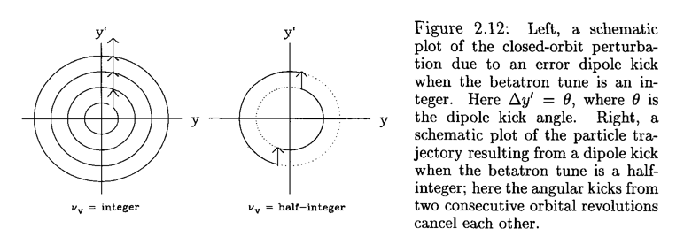
\begin{align} x_{co}&=\sqrt{\beta\left(s\right)}\sum_{m=-\infty}^{\infty} \frac{\nu^2 f_m}{\nu^2-m^2} e^{im\phi(s)} \end{align}We can see clearly that only the harmonic of the error close to the betatron tune will contribute the most on the closed orbit. The following picture shows the comparision of integer and half-integer tune under dipole error.
from map2D import map2D
import numpy as np
import matplotlib.pyplot as plt
#from matplotlib import animation
#from IPython.display import HTML
%matplotlib notebook

dipole_error=map2D(npart=10000, twiss=[2,1], twiss_beam=[2,1],tune=0.228, chrom=10, espr=1e-4)
avex,avep,sizex,sizep,emit=dipole_error.statistics()
emitlist=[]
sizelist=[]
avelist=[]
N_turn=10000

print(dipole_error.linmap)

def evolve_func(turns, kick_turn_start=2000, kick_angle=5e-4,
               ):
    for i in range(turns):
        if i>=kick_turn_start:
            dipole_error.coor2D[1,:]+=kick_angle


        dipole_error.propagate()

        avex,avep,sizex,sizep,emit=dipole_error.statistics()
        avelist.append(avex)
        sizelist.append(sizex)
        emitlist.append(emit)
        yield dipole_error.coor2D

evolve=evolve_func(N_turn+2)

#fig,ax=plt.subplots()
for i in range(N_turn):
    arr=next(evolve)


fig1,(ax1,ax2,ax3)=plt.subplots(3,1, sharex= True)
ax3.set_xlabel("Turns")
ax1.set_ylabel("Centroid [mm]")
ax2.set_ylabel("Beam size [mm]")
ax3.set_ylabel("Emit. [mm mrad]")
ax1.plot(np.array(avelist)*1e3)
ax1.set_ylim([-10,10])
ax2.plot(np.array(sizelist)*1e3)
ax2.set_ylim([0,2])
ax3.set_ylim([0,2])
ax3.plot(np.array(emitlist)*1e6)
fig1.tight_layout()

Perturbed Tune
The gradient error of the quadrupole contribute to the perturbation of the betatron tune. Similar to the dipole errors, we start from the delta function response:
\begin{equation} x''\left(s\right)+\kappa\left(s\right)x\left(s\right)=-(kds)\delta(s-s_0)x(s) \end{equation}We can easily find the tune change from the perturbed matrix as
\begin{align} M_{perturbed}&= M\left(s_{0}\right) \left(\begin{array}{cc} 1 & 0\\ -kds & 1 \end{array}\right)\nonumber\\ &= \left(\begin{array}{cc} \cos\Phi+\alpha_{0}\sin\Phi & \beta_{0}\sin\Phi\\ -\frac{1+\alpha_{0}^{2}}{\beta_{0}}\sin\Phi & \cos\Phi-\alpha_{0}\sin\Phi \end{array}\right) \left(\begin{array}{cc} 1 & 0\\ -kds & 1 \end{array}\right) \nonumber\\ &=\left(\begin{array}{cc} \cos\Phi+\alpha_{0}\sin\Phi-kds\beta_{0}\sin\Phi & \beta_{0}\sin\Phi\\ -\frac{1+\alpha_{0}^{2}}{\beta_{0}}\sin\Phi-kds(\cos\Phi-\alpha_{0}\sin\Phi)& \cos\Phi-\alpha_{0}\sin\Phi \end{array}\right) \end{align}Treat the tune change to be small, therefore the phase advance change is given by
\begin{align} \Delta \Phi &\approx-\frac{\cos\Phi_n-\cos\Phi}{\sin\Phi} \nonumber\\ &=\frac{1}{2}\beta_0 k ds \end{align}Therefore the tune shift is just:
\begin{align} \Delta \nu= \frac{1}{4\pi}\oint \beta(s)k(s)ds \end{align}Consider the location $s_1$, the one turn matrix can be found as:
\begin{align} M(s_1)=M(s_1,s_0)M(s|_0)M(s_0,s_1) \end{align}The change of $m_{12}$ element of $M(s_1)$ is:
\begin{align} \Delta m_{12}=-kds\beta_0\beta_1\sin(\psi_0-\psi_1) \sin(2\pi\nu_0+\psi_1-\psi_0) \end{align}The change of the beta function at $s_1$ is simply:
\begin{align} \Delta \beta_1&=\frac{1}{\sin\Phi}\left(\Delta m_{12}-\beta_1\cos\Phi\Delta\Phi \right) \end{align}Therefore the beta function error gives:
\begin{align} \frac{\Delta \beta_1}{\beta_1}&=\frac{-1}{2\sin\Phi}\int_{s}^{s+C} k(s_0)\beta(s_0) \cos\left(\psi\left(s\right)-\psi\left(s_{0}\right)+2\pi\nu\right) ds_0 \end{align}Follow the similar procedure as in the orbit error, define the Fourier sequence of the quad errors:
\begin{align} \beta^{2}(\phi)k(\phi)=\sum_{m=-\infty}^{\infty}f_m e^{im\phi} \end{align}we have:
\begin{align} \frac{\Delta \beta}{\beta}=-\frac{1}{2}\sum_{m=-\infty}^{\infty} \frac{\nu^2 f_m}{\nu^2-(m/2)^2} e^{im\phi(s)} \end{align}Note that the half integer tune is not stable under the quadrupole errors.
from map2D import map2D
import numpy as np
import matplotlib.pyplot as plt
#from matplotlib import animation
#from IPython.display import HTML
%matplotlib notebook

quad_error=map2D(npart=10000, twiss=[2,1], twiss_beam=[2,1],tune=0.5005, chrom=5.0, espr=1.0e-4)
avex,avep,sizex,sizep,emit=quad_error.statistics()
emitlist=[]
sizelist=[]
avelist=[]
N_turn=6000


def evolve_func(turns, kick_turn_start=1000, df=1.0e-3,
               ):
    for i in range(turns):
        if i>=kick_turn_start:
            quad_error.coor2D[1,:]+=df*quad_error.coor2D[0,:]


        quad_error.propagate()

        avex,avep,sizex,sizep,emit=quad_error.statistics()
        avelist.append(avex)
        sizelist.append(sizex)
        emitlist.append(emit)
        yield quad_error.coor2D

evolve=evolve_func(N_turn+2)

for i in range(N_turn):
    arr=next(evolve)

fig1,(ax1,ax2,ax3)=plt.subplots(3,1, sharex= True)
ax3.set_xlabel("Turns")
ax1.set_ylabel("Centroid [mm]")
ax2.set_ylabel("Beam size [mm]")
ax3.set_ylabel("Emit. [mm mrad]")
ax1.plot(np.array(avelist)*1e3)
ax1.set_ylim([-2,2])
ax2.plot(np.array(sizelist)*1e3)

ax2.set_ylim([0,10])
ax3.set_ylim([0,2])
ax3.plot(np.array(emitlist)*1e6)
fig1.tight_layout()
