Math Review
Linear Algebra
Linear relation can be expressed by $m\times n$ matrix to connect the input of dimension $m$ and response of dimension $n$:
\begin{align} A=\left(\begin{array}{cccc} a_{11} & a_{12} & \cdots & a_{1m}\\ a_{21} & a_{22} & \cdots & a_{2m}\\ \vdots & \vdots & \ddots & \vdots\\ a_{n1} & a_{n2} & \cdots & a_{nm} \end{array}\right) \end{align}Linear properties
If $A$ and $B$ are two matrices with same size $m\times n$, the sum of the two matrices C is the same size with
\begin{equation} C=A+B=B+A \end{equation}\begin{equation} C_{ij}=A_{ij}+B_{ij} \end{equation}The matrix can be scaled by a constant number $k$, aka, scalar multiplication.
\begin{equation} C=kA=Ak \end{equation}\begin{equation} C_{ij}=k A_{ij} \end{equation}Matrix $A$ of size $m\times n$ as its transpose $A^T$:
\begin{equation} A_{ij}^T=A_{ji} \end{equation}Matrix multiplication
Two matrices, $A$ with size $m\times n$ and $B$ with $n\times p$ can be multiplied using matrix multiplication to get $C$ with size of $m\times p$:
\begin{equation} C=AB \end{equation}\begin{equation} C_{ij}=\sum_{k=1}^{n}A_{ik}B_{kj} \end{equation} In general $AB\ne BA$, even if both multiplications are defined
Square matrix
When the size of the two dimensions are same, the matrix is square matrix:
\begin{align} A=\left(\begin{array}{cccc} a_{11} & a_{12} & \cdots & a_{1n}\\ a_{21} & a_{22} & \cdots & a_{2n}\\ \vdots & \vdots & \ddots & \vdots\\ a_{n1} & a_{n2} & \cdots & a_{nn} \end{array}\right) \end{align}A is a square matrix of size $N$.
Diagonal matrix
If the element of a square matrix $A$ $a_{ij}$ are zeros for all $i\ne j$, A is a diagonal matrix.
\begin{align} A=\left(\begin{array}{cccc} a_{11} & 0 & \cdots & 0\\ 0 & a_{22} & \cdots & 0\\ \vdots & \vdots & \ddots & \vdots\\ 0 & 0 & \cdots & a_{nn} \end{array}\right) \end{align}If A and B are all diagonal matrices, the multiplication is commutative:
\begin{align} AB=BA \end{align}A special case of diagonal matrix is unit matrix $I$:
\begin{align} I=\left(\begin{array}{cccc} 1 & 0 & \cdots & 0\\ 0 & 1 & \cdots & 0\\ \vdots & \vdots & \ddots & \vdots\\ 0 & 0 & \cdots & 1 \end{array}\right) \end{align}It is the matrix version of 1 in real number, which satisfies:
\begin{align} AI=IA=A \end{align}Trace of square matrix
The trace of a square matrix $A$ is:
\begin{align} \DeclareMathOperator{\Tr}{Tr} \Tr{A}=\sum_{i=1}^{n}A_{nn} \end{align}Apparently, trace operator is linear:
\begin{align} \DeclareMathOperator{\Tr}{Tr} \Tr{\left(\alpha A + \beta B\right)}=\alpha \Tr{A} + \beta \Tr {B} \end{align}And,
\begin{align} \DeclareMathOperator{\Tr}{Tr} \Tr{AB}=\Tr{BA} \quad\text{even when } AB\ne BA \end{align}In general, trace of matrix multiplication is constant under cyclic permutation:
\begin{align} \DeclareMathOperator{\Tr}{Tr} \Tr{\left(A_1A_2\cdots A_n\right)}=\Tr{\left(A_nA_1A_2\cdots A_{n-1}\right)}= \cdots=\Tr{\left(A_2A_3\cdots A_{n}A_{1}\right)} \end{align}Determinant of square matrix
A square matrix has a quantity called determinant. If the the determinant is non zero, $\det{A}\ne 0$, the matrix is invertible and its invert matrix:
\begin{align} AA^{-1}=A^{-1}A=I \end{align}For $2\times 2$ matrix, the determinant is calculated by:
\begin{align} \det{\left(\begin{array}{cc} a & b \\ c & d \end{array}\right)} =ad-bc \end{align}The determinant has the following property on a $n\times n$ square matrix:
\begin{align} &\det A=\det A^T\\ &\det \left(kA\right)=k^n A \\ &\det \left(AB\right)=\det{A}\det{B} \end{align}Eigensystems of square matrix
If we can find a number $\lambda$ and a non-zero vector $X$ for a square matrix $A$ with size $N$ and satisfy:
\begin{align} AX=\lambda X \end{align}or:
\begin{align} \left(A-\lambda I\right)X=0 \end{align}which requires $\det\left(A-\lambda I\right)=0$, which is a $n^{\text{th}}$ order polynomial.
If the polynomial can be factorized by $\prod_i^N\left(\lambda-\lambda_i\right)=0$, the $\lambda_i$s are the eigenvalues of the matrix $A$. If we can find $N$ independent vectors $X_i$, the matrix $A$ can be be expressed using eigenvalue decomposition:
\begin{align} Q^{-1}AQ=\Lambda \end{align}where,
\begin{align} Q&=\left(\begin{array}{cccc} X_1 & X_2 & \cdots & X_N \end{array}\right) \\ A&=\left(\begin{array}{cccc} \lambda_1 & 0 & \cdots & 0\\ 0 & \lambda_2 & \cdots & 0\\ \vdots & \vdots & \ddots & \vdots\\ 0 & 0 & \cdots & \lambda_N \end{array}\right) \end{align}Primer of Relativistic Mechanics
When object 's speed is comparable to the speed of light, we need to use relativistic mechanics to describe the motion of the object.
The relativistic factors are defined as:
The momentum of the particle, instead of $\mathbf{P}=m\mathbf{v}$, we have
\begin{align} \mathbf{P}=\gamma m\mathbf{v} \end{align}This can be viewed as the mass of the object is 'heavier' by factor of $\gamma$.
The energy of the object reads:
\begin{align} E&=\sqrt{P^2c^2+\left(mc^2\right)^2}\\ &=\gamma m c^2 \end{align}Lorentz transformation
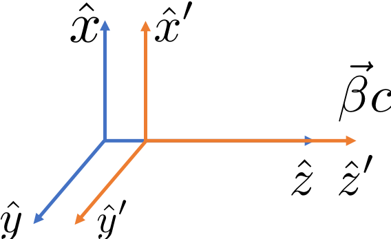
If the coordinate system $K'$ is moving away from the system $K$ with velocity $\boldsymbol{\beta}c$, where the velocity direction is along the $z$ direction. The coordinates of both systems is linked with:
\begin{align} x'&=x\\ y'&=y\\ z'&=\gamma\left(z-\beta c t\right)\\ t'&=\gamma\left(t-\beta z/c\right) \end{align}or in matrix form:
\begin{align} \left(\begin{array}{c} x'\\ y'\\ z'\\ ct' \end{array}\right)=\left(\begin{array}{cccc} 1 & 0 & 0 & 0\\ 0 & 1 & 0 & 0\\ 0 & 0 & \gamma & -\gamma\beta\\ 0 & 0 & -\gamma\beta & \gamma \end{array}\right)\left(\begin{array}{c} x\\ y\\ z\\ ct \end{array}\right) \end{align}Time dilation
Time dilation is the result of Lorentz transformation. Two events happens $\Delta t$ apart at same location in reference frame $K$. If the observer is in the Lorentz boosted frame $K'$, the time difference is
\begin{align} \Delta t'=\gamma \Delta t \end{align}Length contraction.
If an object is at rest in frame $K$ and has length $L$ in $z$ direction, the observer is measuring the length of that object in frame $K'$ by measure both ends of that object simultaneously ($\Delta t'=0$).
Using the invert Lorentz transformation:
\begin{align} L=\Delta z=\gamma \Delta z'+ \gamma\beta c \Delta t' \end{align}Therefore the measured length is:
\begin{align} \Delta z' = \frac{L}{\gamma} \end{align}4-Vector and Lorentz invariant
Lorentz transformation links a space-like variable and a time-like variable. Therefore define a 4-vector can be very useful. The common examples are
- time-space four vector:
- energy-momentum vector
- electromagnetic four-potential
The dot product of two four vectors $A=(a_0,a_1,a_2,a_3)$ and $B=(a_0,a_1,a_2,a_3)$ are defined as:
\begin{equation} A\cdot B=\left(\begin{array}{c} a_{0}\\ a_{1}\\ a_{2}\\ a_{3} \end{array}\right)^{T}\left(\begin{array}{cccc} 1 & 0 & 0 & 0\\ 0 & -1 & 0 & 0\\ 0 & 0 & -1 & 0\\ 0 & 0 & 0 & -1 \end{array}\right)\left(\begin{array}{c} b_{0}\\ b_{1}\\ b_{2}\\ b_{3} \end{array}\right) \end{equation}It can be prove that the dot product of two 4-vectors is an invaiant under Lorentz transformtion.
Differential Equation
Here, we limit our discussion to oridnary differential equation of the first order and second order. Here are some examples:
- First order homogeneous equation
- First order inhomogeneous equation
- Second order homogeneous equation
- Second order inhomogeneous equation
Harmonic oscillator
The motion of harmonic oscillator satisfy a second order differential equation.
\begin{align} \frac{d^2x}{dt^2}+\omega^2 x=0 \end{align}The solution to the equation is
\begin{align} x=Ae^{i\omega t}+Be^{-i\omega t} \end{align}Here the constant $A$ and $B$ has to be determined by initial condition, e.g. the $x(t=0)$ and $x'(t=0)$. Alternatively the solution can be written as:
\begin{align} x=A\cos\left(\omega t+\phi_0\right) \end{align}import numpy as np
import matplotlib.pyplot as plt
%matplotlib notebook
fig,ax=plt.subplots()
omega=5
t=np.linspace(0,10, 1000)
x=np.cos(omega*t)
ax.set_xlabel('Time')
ax.set_ylabel('Osci. amplitude')
ax.plot(t,x)
pass

Damped Harmonic oscillator
If damping effect exist in the oscillator, the motion is described by the differential equation:
\begin{align} \frac{d^2x}{dt^2}+2\alpha\frac{dx}{dt}+\omega^2 x=0 \end{align}The solution is given by: The solution to the equation is
\begin{align} x=Ae^{i\lambda_1 t}+Be^{i \lambda_2 t} \end{align}where
\begin{align} \lambda_{1/2}=-\alpha\pm i \sqrt{\omega^2-\alpha^2} \end{align}In accelerator, we almost always have weak damping effect only, i.e. $\omega \gg \alpha$
import numpy as np
import matplotlib.pyplot as plt
%matplotlib notebook
fig,ax=plt.subplots()
omega=5
damp=0.1
t=np.linspace(0,10, 1000)
x=np.exp(-damp*t)*np.cos(np.sqrt(omega*omega-damp*damp)*t)
ax.set_xlabel('Time')
ax.set_ylabel('Osci. amplitude')
ax.plot(t,x)
ax.plot(t,np.exp(-damp*t), '--', alpha=0.5)
pass

Vector Operation
Accelerator science deals the charged particle motion in E-M field. Therefore Maxwell equation is our starting point of many problems.
Differential Form |
Integral From |
|
|---|---|---|
| Gauss Law | $\nabla\cdot\mathbf{E} = \frac{\rho}{\varepsilon_0}$ | $\oint \mathbf{E} d\mathbf{S}=\frac{1}{\varepsilon_0}\iiint \rho dV$ |
| $\nabla\cdot\mathbf{B} = 0$ | $\oint \mathbf{B} d\mathbf{S}=0$ | |
| Faraday's Law | $\nabla\times\mathbf{E} =-d\mathbf{B}/{dt}$ | $\oint \mathbf{E}d\mathbf{l}=-\frac{d}{dt}\oint \mathbf{B} d\mathbf{S}$ |
| Ampere's Law | $\nabla \times \mathbf{B} = \mu_0\left(\mathbf{J} + \varepsilon_0 \frac{\partial \mathbf{E}} {\partial t} \right)$ | $\oint \mathbf{B}d\mathbf{l}=\mu_0\left(\oint\mathbf{J}d\mathbf{S}+\varepsilon_0\frac{d}{dt}\oint \mathbf{E} d\mathbf{S}\right)$ |
Therefore the vector operations are frequently used.
Gradient, Divergence and Curl
- Gradient of scalar function is a vector
- Divergence of a vector is a scalar function
- Curl of the vector is another vector function
Gauss's divergence theorem
\begin{align} \int_S \mathbf{f}\cdot d\mathbf{S}=\int_V \nabla\cdot\mathbf{f}dV \end{align}It is useful to find the electric field with given charge distribution.
Stokes' theorem
\begin{align} \int_{S} \nabla \times \mathbf{f} \cdot d\mathbf{S} = \oint_{\partial S} \mathbf{f} \cdot d \mathbf{r} \end{align}It is useful to find the magnetic field with given current distribution.
Example: Gradient of a 2D potential
import matplotlib.pyplot as plt
import numpy as np

x1=3.45;y1=-3.38;c1=-0.7
x2=-2.48;y2=2.96;c2=1.2
x3=4.47;y3=3.7;c3=-0.5

xlist=np.linspace(-5,5,500)
ylist=np.linspace(-5,5,500)

xx, yy = np.meshgrid(xlist, ylist, sparse=False, indexing='ij')
r1sqr=(xx-x1)**2+(yy-y1)**2
r2sqr=(xx-x2)**2+(yy-y2)**2
r3sqr=(xx-x3)**2+(yy-y3)**2

potential=-c1*np.log(r1sqr)/2-c2*np.log(r2sqr)/2-c3*np.log(r3sqr)/2
ex=np.zeros_like(potential)
ey=np.zeros_like(potential)
ex[1:-1,1:-1]=(potential[2:, 1:-1]-potential[0:-2, 1:-1])/2
ey[1:-1,1:-1]=(potential[1:-1, 2:]-potential[1:-1, 0:-2])/2

fig, (ax1,ax2)=plt.subplots(1,2)
ax1.set_aspect('equal');ax2.set_aspect('equal')
ppot =ax1.contour(xx,yy, potential, [-5, -3, -1.5, -1,-0.5, 0, 0.5,1, 1.5, 3, 5])
skip=24
ax2.quiver(xx[1:-1:skip,1:-1:skip], yy[1:-1:skip,1:-1:skip], ex[1:-1:skip,1:-1:skip], ey[1:-1:skip,1:-1:skip])
ax1.clabel(ppot, inline=1, fontsize=10)
plt.show()
