Transverse Dynamics
Transverse dynamics of accelerator focuses on the dynamics of transporting the charged particle to a specific location (transport line) or with periodic boundary condition (a accelerator ring).
To affect the motion of a charged particle, we need external magnetic field or electric field, followed by the Lorentz force:
\begin{align} \mathbf{F}=q\left(\mathbf{E}+\mathbf{v}\times\mathbf{B}\right) \end{align}Magnetic or Electric Fields?
To have the same Lorentz force on the charged particle, the comparable magnetic field and electric field is scaled by velocity of the particle. The below table lists the electric field need to have same force of 1 Tesla magnetic field.
| $\gamma-1=\frac{E_k}{E_0}$ | $\beta c$ | $\mathbf{B}$ (T) | $\mathbf{E}$ (MV/m) |
|---|---|---|---|
| $10^{-5}$ | 0.0045$c$ | 1 | 1.34 |
| $10^{-4}$ | 0.0141$c$ | 1 | 4.24 |
| $10^{-3}$ | 0.0447$c$ | 1 | 13.4 |
| $10^{-2}$ | 0.140$c$ | 1 | 42.1 |
| $10^{-1}$ | 0.417$c$ | 1 | 125 |
Considering the field break down limit of the electric field, we see that only when the particle velocity is not relativistic, the electric field can be used. Therefore the magnetic field is widely used to bend/steer/focus the relativistic particles.
Design Orbit and Coordinate System
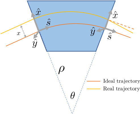
The geometry of the accelerator is determined by the dipole magnet. Let us assume that the magnetic field is constant in certain region and along the vertical direction $\mathbf{B}=B_0\hat{y}$. The particle travels through this region initially in $\hat{s}$ direction in the $x$-$s$ plane, as shown below.
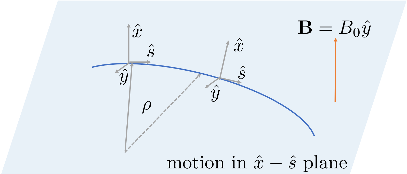
Note that the coordinate moves along the ideal beam trajectory and the $\hat{s}$ is always along the tangent direction and $\hat{x}$ is pointing against the normal direction. This is named Frenet–Serret coordinate system.
The equation of motion is
\begin{equation} \frac{d\mathbf{P}}{dt}=q\mathbf{v}\times\mathbf{B} \end{equation}The momentum change will be only in the $x$-$s$ plane, the velocity is always perpendicular to the magnetic field and the energy of the beam does not change, therefore:
\begin{equation} m\gamma \frac{d\mathbf{v}}{dt}=qB_0\mathbf{v}\times\hat{y} \end{equation}Using the fact that the amplitude of the velocity will not change therefore:
\begin{equation} m\gamma \frac{v^2}{\rho}=qvB_0 \end{equation}The bending radius is given by:
\begin{equation} \rho=\frac{\left|\mathbf{P}\right|}{qB_0} \end{equation}Here, we define the term 'rigidity' $B_0\rho=P/q$, to quantify 'how hard to bend the beam'. And naturally it is only function of the particle momentum amplitude. It is a very important normalization factor of the transverse motion, as will shown later. After normalization, most our calculation becomes particle energy independent.
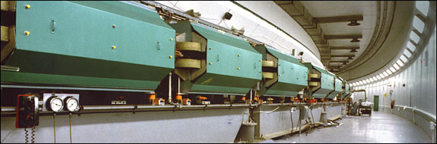
The dipoles that defines the geometry of the accelerator are sometimes called main dipoles. They define a ideal trajectory. A charge particle with correct energy, once inject with correct position and angle, will exactly follow the ideal trajectory.
Magnetic Multi-poles
There are many common type of magnets used accelerators, they are grouped using the order of multi-pole expansion in the vicinity of the center of the beam pipe, where the particles is transported. Here are the list of common type of magnets
| Magnet Types | Usages |
|---|---|
| Dipoles | Form the Geometry of Accelerator |
| Quadrupoles | Focus/Defocus the beam |
| Sextrupole | Chromatic correction, nonlinear effects |
| Octopole | Damping of the collective effects |
| Solenoid | Focusing for low energy beam |
| Correctors | Steer the beam |
In a vacuum chamber, the region is sourceless, i.e. there is no charge or current. The magnet field can be expressed using 'Beth representation':
\begin{align} B_y+iB_x &= B_0 \sum_{n=0}^\infty \left(b_n + i a_n\right) \left(x+iy\right)^{n} &&\quad\text{(U.S. convention)}\\ &= B_0 \sum_{m=1}^\infty \left(b_m + i a_m\right) \left(x+iy\right)^{m-1} &&\quad\text{(European convention)} \end{align}Here, $B_0$ is the main dipole field strength. The $b_n$ and $a_n$ are called the $2(n+1)^{th}$ multipole coefficients in 'U.S. convention' (starting from $n=0$); while the $b_m$ and $a_m$ are called $2m^{th}$ multipole coefficients in 'European convention' (starting from $m=1$). The set of $b$ coefficients are the normal components while the set of $a$ coefficients are the skew components.
To achieve high field, accelerator usually use high permeability material to boost the flux density $\mathbf{B}$ for the same magnetic field generated by the coil.
\begin{equation} \mathbf{B}=\mu_r \mu_0 \mathbf{H} \end{equation}The figure below shows the permeability of ferromagnet material as function of the external magnetic field $\mathbf{H}$:

In the magnet design, we use iron cores as the ferromagnet materials. iron (99.8% pure) may have initial $\mu_r$ of 150 and can reach maximum of 5000; while the %99.95 pure ion will have initial $\mu_r$ of 10000 and reach maximum 200000.
At such high permeability, the magnetic field line is always perpendicular to the surface of the iron core.
Dipole
If only the lowest order of coefficient are non-zero values, the field reads:
\begin{align} B_y&=B_0 b_0 \\ B_x&=B_0 a_0 \end{align}in US convention.
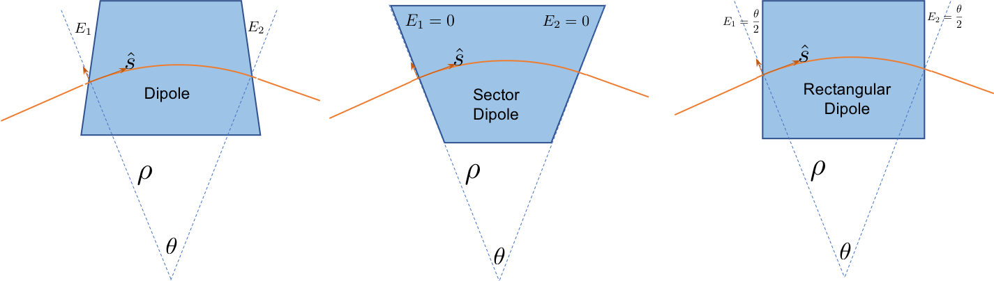
The main dipoles will have $b_0=1$ and $a_0=0$. Below, two types of dipoles magnet are shown in the cartoon:
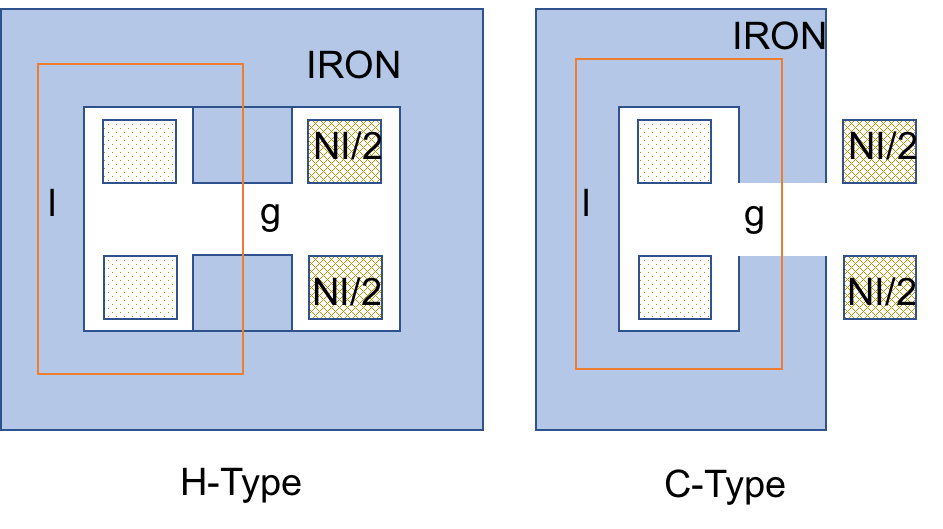
Since the dipole bend the ideal trajectory. The both edges of the dipoles may affect the motion of the particle. Below, dipole with general edge angle is shown. The most useful types are sector dipoles, with zero edge angles on each side and rectangular dipoles who has both edge angles equaling the half of the bending angle.
Quadrupole
The magnet is named quadrupole when the quad coefficient $b_1$ and/or $a_1$ are non-zero (US convention). They are named normal quadrupole and skew quadrupole accordingly. The field line of the quadrupole are:
import numpy as np
import matplotlib.pyplot as plt
%matplotlib notebook
fig, (ax1,ax2)=plt.subplots(1,2)
ax1.set_aspect('equal');ax2.set_aspect('equal')
xlist = np.linspace(-5.0, 5.0, 40)
ylist = np.linspace(-5.0, 5.0, 40)
X, Y = np.meshgrid(xlist, ylist)
Zn = X*Y
Zs = (X*X-Y*Y)/2

ax1.set_title('Normal Quad', )
ax2.set_title('Skew Quad', )
ax1.set_xlabel('x')
ax2.set_xlabel('x')
ax1.set_ylabel('y')
cp_n =ax1.contour(X, Y, Zn, [-6,-4,-2,2,4,6])
cp_s =ax2.contour(X, Y, Zs, [-6,-4,-2,2,4,6])
ax1.quiver(X[::3,::3], Y[::3,::3], Y[::3,::3], X[::3,::3])
ax2.quiver(X[::3,::3], Y[::3,::3], X[::3,::3], -Y[::3,::3])
ax1.clabel(cp_n, inline=True, fontsize=3)
ax2.clabel(cp_s, inline=True, fontsize=3)
pass

The normal quadrupole has the magnetic field as:
\begin{equation} \mathbf{B}=B_0 b_1\left(y \hat{x}+x \hat{y}\right) \end{equation}while the skew quadrupole has the magnetic field as:
\begin{equation} \mathbf{B}=B_0 a_1\left(x \hat{x}-y \hat{y}\right) \end{equation}Sextrupole
The magnet is named Sextrupole when the sextrupole coefficient $b_2$ and/or $a_2$ are non-zero (US convention). They are named normal sextrupole and skew sextrupole accordingly. The field line of the sextrupole are:
fig, (ax1,ax2)=plt.subplots(1,2)
ax1.set_aspect('equal');ax2.set_aspect('equal')
xlist = np.linspace(-5.0, 5.0, 40)
ylist = np.linspace(-5.0, 5.0, 40)
X, Y = np.meshgrid(xlist, ylist)
Zn = (3*X*X*Y-Y*Y*Y)/3
Zs = (X*X*X-3*X*Y*Y)/3

ax1.set_title('Normal Sextrupole', )
ax2.set_title('Skew Sextrupole', )
ax1.set_xlabel('x')
ax2.set_xlabel('x')
ax1.set_ylabel('y')
cp_n =ax1.contour(X, Y, Zn, np.array([-6,-4,-2,2,4,6])*3)
cp_s =ax2.contour(X, Y, Zs, np.array([-6,-4,-2,2,4,6])*3)
ax1.quiver(X[::3,::3], Y[::3,::3], (2*X*Y)[::3,::3], (X*X-Y*Y)[::3,::3])
ax2.quiver(X[::3,::3], Y[::3,::3], (X*X-Y*Y)[::3,::3], (-2*X*Y)[::3,::3])
ax1.clabel(cp_n, inline=True, fontsize=3)
ax2.clabel(cp_s, inline=True, fontsize=3)

The normal sextrupole has the magnetic field as:
\begin{equation} \mathbf{B}=B_0 b_2\left[2xy \hat{x}+\left(x^2-y^2\right) \hat{y}\right] \end{equation}while the skew Sextrupole has the magnetic field as:
\begin{equation} \mathbf{B}=B_0 a_2\left[\left(x^2-y^2\right) \hat{x}- 2xy\hat{y}\right] \end{equation}Linear Transverse Motion
Motion in Quadrupole
The simplest motion of the charged particle is in normal quadrupole, whose field is
\begin{align} B_x&=Gy\\ B_y&=Gx \end{align}where the gradient is $G=B_0 b_1$.
Quadrupole is usually positioned so that the zero field axis is located on the ideal trajectory. The ideal particle will not experience any field from the Quadrupole.
From the Lorentz force, we have $$\gamma m \frac{d\mathbf{v}}{dt} = q \mathbf{v}\times \mathbf{B}$$
Expand the vector production and get
\begin{align} \gamma m\frac{d^{2}x}{dt^{2}}&=-qGxv_{z}\\ \gamma m\frac{d^{2}y}{dt^{2}}&=qGyv_{z} \end{align}Here we need to make following approximation:
- paraxial approximation, indicate that the particle will only deviate the design direction by small angles, i.e. if z is the forward direction, the two transverse velocity satisfy: $v_x,v_y \ll \left|\mathbf{v}\right|$
- In such approximation,
- Using such approximation, we have $$\frac{d}{dt}=v_s\frac{d}{ds}\sim v\frac{d}{ds}\;\frac{d^2}{dt^2}\sim v^2\frac{d^2}{ds^2}$$
Then the equation of motion in quadrupole is simplified as
\begin{align} \gamma m v\frac{d^{2}x}{ds^{2}}&=qGx\\ \gamma m v\frac{d^{2}y}{ds^{2}}&=-qGy \end{align}Using the definition of the rigidity $B\rho$, the EOM can be rewritten as :
\begin{align} \frac{d^{2}x}{ds^{2}}&=-\frac{G}{B\rho}x\\ \frac{d^{2}y}{ds^{2}}&=\frac{G}{B\rho}y \end{align}Then, we define the normalized quadrupole strength $k=G/(B\rho)$, the EOM is simply:
\begin{align} \frac{d^{2}x}{ds^{2}}+kx&=0\\ \frac{d^{2}y}{ds^{2}}-ky&=0 \end{align}In later syntax, we use prime ($'$) to denote the derivative with respective to $s$.
Depend on the sign of $k$, it is easy to solve the differential equation:
\begin{equation} x\left(s\right)= \begin{cases} a \cos \left(\sqrt{k}s\right)+b \sin \left(\sqrt{k}s\right)&k>0\\ a s + b &k=0\\ a \cosh \left(\sqrt{-k}s\right)+b\sinh \left(\sqrt{-k}s\right)&k<0 \end{cases} \end{equation}The three cases corresponds to a focusing quadrupole, drift space and a defocusing quadrupole respectively. The parameter $a$, $b$ are determined by the initial particle position $x$ and its derivative $x'$. We also learn that the quadrupole will always focus the particles in one transverse direction and defocus in the other.
Motion in Dipole
Dipole itself will not affect the beam other than bending. However, the choice of the Frenet–Serret system results a focusing effect in kinetics, as shown in the above figure.
If the particle is injected $x$ (>0) away from the ideal trajectory, the particle will travel longer in the dipole than the ideal particle, which results a larger bending. When the bending angle $\theta$ is small, we have:
\begin{align} \Delta x'&= -\frac{x}{\rho} \theta = -\frac{x}{\rho^2} \Delta s\\ \Delta y'&= 0 \end{align}Therefore the particle satisfy the following differential equation in dipole:
\begin{align} &x''+\frac{1}{\rho^2} x =0\\ &y''=0\\ \end{align}And the solution of the equation of motion is simply:
\begin{align} x(s)&=a \cos \left(\frac{s}{\rho}\right)+b \sin \left(\frac{s}{\rho}\right) \\ y(s)&=a s + b \end{align}Hill's Equation
Let's combine the effects of the dipole and quadrupole and write the equation of motion as the form of Hill's equation:
\begin{align} &x''+\left(\frac{1}{\rho^2(s)} + k(s)\right)x =0\\ &y''-k(s) y=0\\ \end{align}In general, the radius $\rho$ and focusing strength $k$ are function of the longitudinal coordinate $s$. If the parameter is piecewise constant, we can solve it as we did in the last two sections.
Transverse Matrix
It is convenient to write the solution of the Hill's equation using matrix form. Such matrix is named betatron transfer matrix. The motion in each transverse direction passing through a specific magnet can be described by $2\times 2$ matrix $M$,
\begin{equation} M=\left(\begin{array}{cc} m_{11} & m_{12}\\ m_{21} & m_{22} \end{array}\right) \end{equation}as:
\begin{equation} \left(\begin{array}{c} x\\ x' \end{array}\right)_{\text{exit}}=M\left(\begin{array}{c} x\\ x' \end{array}\right)_{\text{entrance}} \end{equation}Drift space
The EOM for drift space is simply $x''=0$ and $y''=0$. Using horizontal direction as instance, if the initial condition at the starting point $s_0$ are $x(s=s_0)=x_0$ and $x'(s=s_0)={x_0'}$. The solution is:
\begin{equation} x(s=s_0+l)=x_0+x'_0l \end{equation}Or in matrix form
\begin{equation} \left(\begin{array}{c} x\\ x' \end{array}\right)_{s=s_0+l}=\left(\begin{array}{cc} 1 & l\\ 0 & 1 \end{array}\right)\left(\begin{array}{c} x\\ x \end{array}\right)_{s=s_0} \end{equation}We write the transfer matrix for drift space as:
\begin{equation}M\left(s_0+s,s_0\right)=\left(\begin{array}{cc} 1 & s\\ 0 & 1 \end{array}\right) \end{equation}Below is an example to illustrate the particle distribution and trajectory of a drift space of 2 meters. The main windows shows trajectory of each particle, the inlets display the distribution at either end of the drift space.
import numpy as np
import matplotlib.pyplot as plt

num_par=1000
xsize=1  # mm
pxsize=0.999 # mrad
coor=-1
distance=2
coor=-1/np.sqrt(xsize*xsize/pxsize/pxsize-1)  # create the waist at s=0

step=1
dot_size_scale=np.log(2*num_par)**1.2
mod_xsize=xsize/np.sqrt(1+coor*coor)
beta=mod_xsize/pxsize
virtual_drift=coor*beta

particle_coor=np.zeros((3*step+3, num_par))
particle_coor[0, :]=np.random.randn(num_par)*mod_xsize
particle_coor[1, :]=np.random.randn(num_par)*pxsize
particle_coor[0, :]+=particle_coor[1, :]*virtual_drift
particle_coor[2, :]=np.zeros(num_par)-1.0

particle_coor[3, :]=particle_coor[0, :]+particle_coor[1, :]*distance
particle_coor[4, :]=particle_coor[1, :]
particle_coor[5, :]=particle_coor[2, :]+distance

max_x=np.max([np.max(particle_coor[[0,3], :])*1.1, 3*xsize])
max_px=np.max([np.max(particle_coor[[1,4], :])*1.1, 3*pxsize])
fig,ax=plt.subplots(figsize=(8,6))
ax.set_xlim(-1.5,1.5)
ax.set_ylim(-max_x,max_x*1.6)
ax.plot(particle_coor[[2,5],:],particle_coor[[0,3],:], lw=2/dot_size_scale)
ax.set_xlabel("Longitudinal position [m]")
ax.set_ylabel("Transverse position [mm]")
ax.axvline(x=1,ymin=.5, ymax=2/2.6, linestyle='-.', lw=1, alpha=.6)
ax.axvline(x=-1,ymin=.5, ymax=2/2.6, linestyle='-.', lw=1, alpha=.6)
axins1 = ax.inset_axes([0.02, 0.68, 0.3, 0.3])
axins1.set_xlim([-max_x,max_x])
axins1.set_ylim([-max_px,max_px])
axins1.plot(particle_coor[0,:], particle_coor[1,:],ls='None',marker='.', ms=6/dot_size_scale)
axins1.set_xticks([])
axins1.set_yticks([])

axins2 = ax.inset_axes([0.68, 0.68, 0.3, 0.3])
axins2.plot(particle_coor[3,:], particle_coor[4,:],ls='None',marker='.', ms=6/dot_size_scale)
axins2.set_xlim([-max_x,max_x])
axins2.set_ylim([-max_px,max_px])
axins2.set_xticks([])
axins2.set_yticks([])
plt.show()

Dipoles
For the dipole that bend the beam with the radius $\rho$ in horizontal plane, the $x$ direction follows an EOM as a harmonic oscillator, while in $y$ direction, the motion is just as in a drift space.
The matrix form in the dipole can be easily get as:
\begin{equation} \left(\begin{array}{c} x\\ x' \end{array}\right)_{s=s_0+l}=\left(\begin{array}{cc} \cos(l/\rho) & \rho\sin(l/\rho)\\ -\sin(l/\rho)/\rho & \cos(l/\rho) \end{array}\right)\left(\begin{array}{c} x\\ x \end{array}\right)_{s=s_0} \end{equation}The transfer matrix for dipole in horizontal space is:
\begin{equation} M\left(s_0+s,s_0\right)=\left(\begin{array}{cc} \cos\left(\frac{l}{\rho}\right) & \rho\sin\left(\frac{l}{\rho}\right)\\ -\frac{1}{\rho}\sin\left(\frac{l}{\rho}\right) & \cos\left(\frac{l}{\rho}\right) \end{array}\right) \end{equation}In a small angle approximation $s/\rho \ll1$, we can expand the matrix up to first order of $s/\rho$. The matrix reduce to a drift space:
\begin{equation} M\left(s_0+l,s_0\right)=\left(\begin{array}{cc} 1 & l\\ 0 & 1 \end{array}\right) \end{equation}Quadrupoles
In the example before, we already derived the solution for particle in the quadrupole. It can be rewritten in the matrix form as
\begin{equation} M\left(s_0+s,s_0\right)= \begin{cases} \left(\begin{array}{cc} \cos\left(\sqrt{k}s\right) & \sin\left(\sqrt{k}s\right)/\sqrt{k}\\ -\sqrt{k}\sin\left(\sqrt{k}s\right) & \cos\left(\sqrt{k}s\right) \end{array}\right)&k>0, \text{Focusing Quad}\\ \\ \left(\begin{array}{cc} \cosh\left(\sqrt{-k}s\right) & \sinh\left(\sqrt{-k}s\right)/\sqrt{-k}\\ \sqrt{-k}\sinh\left(\sqrt{-k}s\right) & \cosh\left(\sqrt{-k}s\right) \end{array}\right)&k<0, \text{Defocusing Quad}\\ \end{cases} \end{equation}Usually, the quadrupole has short length and strong field gradient. We may model such short quad as a 'lens with zero length', and define the focal length $f$ as:
\begin{equation} f=\lim_{l\to 0}\frac{1}{|k|l} \end{equation}In such limit the transfer map for a thin-length quad is
\begin{equation} M_{\text{quad}}= \begin{cases} \left(\begin{array}{cc} 1 & 0\\ -1/f & 1 \end{array}\right)& \text{Focusing Quad}\\ \\ \left(\begin{array}{cc} 1 & 0\\ 1/f & 1 \end{array}\right)& \text{Defocusing Quad}\\ \end{cases} \end{equation}import numpy as np
import matplotlib.pyplot as plt
num_par=10
xsize=0.8 # mm
pxsize=0.4 # mrad
coor=-0.5
distance=1
focallen=-1
step=2
dot_size_scale=np.log(2*num_par)**1.2
mod_xsize=xsize/np.sqrt(1+coor*coor)
beta=mod_xsize/pxsize
virtual_drift=coor*beta
particle_coor=np.zeros((3*step+3, num_par))
particle_coor[0, :]=np.random.randn(num_par)*mod_xsize
particle_coor[1, :]=np.random.randn(num_par)*pxsize
particle_coor[0, :]+=particle_coor[1, :]*virtual_drift
particle_coor[2, :]=np.zeros(num_par)-1.0
particle_coor[3, :]=particle_coor[0, :]+particle_coor[1, :]*distance
particle_coor[4, :]=particle_coor[1, :]
particle_coor[5, :]=particle_coor[2, :]+distance
particle_coor[7, :]=particle_coor[4, :]+particle_coor[3, :]/focallen
particle_coor[6, :]=particle_coor[3, :]+particle_coor[7, :]*distance
particle_coor[8, :]=particle_coor[5,:]+distance
max_x=np.max([np.max(particle_coor[[0,3,6], :])*1.1, 3*xsize])
max_px=np.max([np.max(particle_coor[[1,4,7], :])*1.1, 3*pxsize])
fig,ax=plt.subplots(figsize=(8,6))
ax.set_xlim(-1.5,1.5)
ax.set_ylim(-max_x,max_x*1.6)
ax.plot(particle_coor[[2,5,8],:],particle_coor[[0,3,6],:], lw=2/dot_size_scale)
ax.axvline(x=1,ymin=2/2.6-0.2, ymax=2/2.6, linestyle='-.', lw=1, alpha=.6)
ax.axvline(x=0,ymin=2/2.6-0.2, ymax=2/2.6, linestyle='-.', lw=1, alpha=.6)
ax.axvline(x=-1,ymin=2/2.6-0.2, ymax=2/2.6, linestyle='-.', lw=1, alpha=.6)
ax.set_xlabel("Longitudinal position [m]")
ax.set_ylabel("Transverse position [mm]")
axins1 = ax.inset_axes([0.02, 0.68, 0.3, 0.3])
axins1.set_xlim([-max_x,max_x])
axins1.set_ylim([-max_px,max_px])
axins1.plot(particle_coor[0,:], particle_coor[1,:],ls='None',marker='.', ms=6/dot_size_scale)
axins1.set_xticks([])
axins1.set_yticks([])
axins2 = ax.inset_axes([0.35, 0.68, 0.3, 0.3])
axins2.plot(particle_coor[3,:], particle_coor[4,:],ls='None',marker='.', ms=6/dot_size_scale)
axins2.set_xlim([-max_x,max_x])
axins2.set_ylim([-max_px,max_px])
axins2.set_xticks([])
axins2.set_yticks([])
axins3 = ax.inset_axes([0.68, 0.68, 0.3, 0.3])
axins3.plot(particle_coor[6,:], particle_coor[7,:],ls='None',marker='.', ms=6/dot_size_scale)
axins3.set_xlim([-max_x,max_x])
axins3.set_ylim([-max_px,max_px])
axins3.set_xticks([])
axins3.set_yticks([])
plt.show()

Chain of linear elements
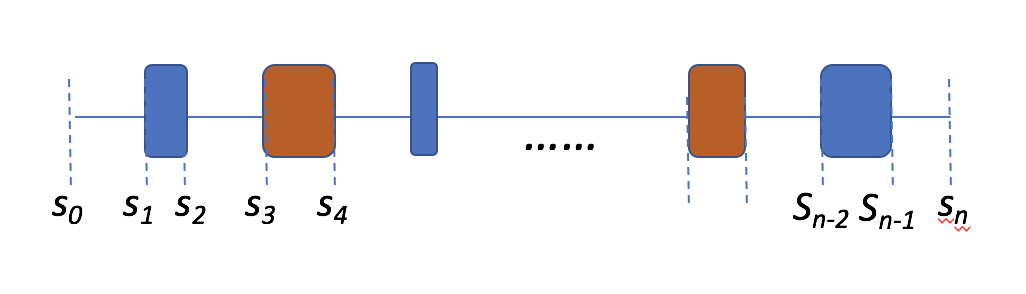
In accelerators, we have chain of magnets, as illustrated above. Each magnet has a transfer matrix, the transfer matrix for the chain can be found by matrix multiplications:
\begin{equation} M\left(s_n,s_0\right)=M\left(s_n,s_{n-1}\right)\cdots M\left(s_2,s_1\right)M\left(s_1,s_0\right) \end{equation}Note that the order of the multiplication is the reverse order of the placement of the magnet.
Usually we call the sequence of the magnets as lattice.
import numpy as np
import matplotlib.pyplot as plt

num_par=1000
xsize=0.8  # mm
pxsize=0.4 # mrad
coor=-1
distance=1
focallen=1.5
coor=-focallen/np.sqrt(focallen*focallen-distance*distance) # coor for matching condition
pxsize=xsize/np.sqrt(2*focallen*focallen-distance*distance)


step=3
dot_size_scale=np.log(2*num_par)**1.2
mod_xsize=xsize/np.sqrt(1+coor*coor)
beta=mod_xsize/pxsize
virtual_drift=coor*beta

particle_coor=np.zeros((3*step+3, num_par))
particle_coor[0, :]=np.random.randn(num_par)*mod_xsize
particle_coor[1, :]=np.random.randn(num_par)*pxsize
particle_coor[0, :]+=particle_coor[1, :]*virtual_drift
particle_coor[2, :]=np.zeros(num_par)-2.0

particle_coor[3, :]=particle_coor[0, :]+particle_coor[1, :]*distance
particle_coor[4, :]=particle_coor[1, :]
particle_coor[5, :]=particle_coor[2, :]+distance


particle_coor[7, :]=particle_coor[4, :]+particle_coor[3, :]/focallen
particle_coor[6, :]=particle_coor[3, :]+particle_coor[7, :]*2*distance
particle_coor[8, :]=particle_coor[5,:]+2*distance

particle_coor[10, :]=particle_coor[7, :]-particle_coor[6, :]/focallen
particle_coor[9, :]=particle_coor[6, :]+particle_coor[10, :]*distance
particle_coor[11, :]=particle_coor[8,:]+distance

max_x=np.max([np.max(particle_coor[[0,3,6,9], :])*1.1, 3*xsize])
max_px=np.max([np.max(particle_coor[[1,4,7,10], :])*1.1, 3*pxsize])
fig,ax=plt.subplots(figsize=(11,6))
ax.set_xlim(-2.5,2.5)
ax.set_ylim(-max_x,max_x*1.6)
ax.plot(particle_coor[[2,5,8,11],:],particle_coor[[0,3,6,9],:], lw=2/dot_size_scale)
ax.axvline(x=-2,ymin=2/2.6-0.2, ymax=2/2.6, linestyle='-.', lw=1, alpha=.6)
ax.axvline(x=-1,ymin=2/2.6-0.2, ymax=2/2.6, linestyle='-.', lw=1, alpha=.6)
ax.axvline(x=1,ymin=2/2.6-0.2, ymax=2/2.6, linestyle='-.', lw=1, alpha=.6)
ax.axvline(x=2,ymin=2/2.6-0.2, ymax=2/2.6, linestyle='-.', lw=1, alpha=.6)
ax.set_xlabel("Longitudinal position [m]")
ax.set_ylabel("Transverse position [mm]")
axins1 = ax.inset_axes([0.01, 0.68, 0.2, 0.3])
axins1.set_xlim([-max_x,max_x])
axins1.set_ylim([-max_px,max_px])
axins1.plot(particle_coor[0,:], particle_coor[1,:],ls='None',marker='.', ms=6/dot_size_scale)
axins1.set_xticks([])
axins1.set_yticks([])

axins2 = ax.inset_axes([0.22, 0.68, 0.2, 0.3])
axins2.plot(particle_coor[3,:], particle_coor[4,:],ls='None',marker='.', ms=6/dot_size_scale)
axins2.set_xlim([-max_x,max_x])
axins2.set_ylim([-max_px,max_px])
axins2.set_xticks([])
axins2.set_yticks([])

axins3 = ax.inset_axes([0.58, 0.68, 0.2, 0.3])
axins3.plot(particle_coor[6,:], particle_coor[7,:],ls='None',marker='.', ms=6/dot_size_scale)
axins3.set_xlim([-max_x,max_x])
axins3.set_ylim([-max_px,max_px])
axins3.set_xticks([])
axins3.set_yticks([])

axins4 = ax.inset_axes([0.79, 0.68, 0.2, 0.3])
axins4.plot(particle_coor[9,:], particle_coor[10,:],ls='None',marker='.', ms=6/dot_size_scale)
axins4.set_xlim([-max_x,max_x])
axins4.set_ylim([-max_px,max_px])
axins4.set_xticks([])
axins4.set_yticks([])

plt.show()

Properties of the transverse matrix
Symplectic condition
The matrix represents the dynamics of charged particle, which obeys the energy conservation law. We claim the property of the matrix due to energy conservation as symplectic condition. In $2\times 2$ matrix case, the symplectic condition becomes:
\begin{equation} \det(M)=1 \end{equation}Long-term stability condition
The symplecticity ensures the area phase space is constant. However, in most times, we have stronger requirements for a repeating chain of elements.
In accelerator, the beam usually will pass through a chain of elements (called cell) many times. A long lattice usually consist of repeating cells. In a ring accelerator, the particle will travels through the lattice billions of turns. If the transfer matrix for one cell is $M$, we are interested in the behavior of repeating $k$ cells $$M_{total}=M\cdot M\cdots M\cdot M=M^k$$ where k is a very large integer or infinity.
To avoid the either $x$ or $x'$ to be very large (or infinity) after k cells. We required that the absolute value of the eigenvalues of $M$ is no larger than 1. The eigenvalue is found by:
\begin{equation} \left|\begin{array}{cc} \lambda-a & -b\\ -c & \lambda-d \end{array}\right|=0 \end{equation}or
\begin{equation} \lambda^2-(a+d)\lambda+1=0 \end{equation}To satisfy $|\lambda|\le 1$, we require
\begin{equation} \left|Tr(M)\right|=\left|a+d\right|\le 2 \end{equation}This is the stable condition for one cell in periodical structure.
Twiss Parametrization
To separate description of transverse motion from contribution the lattice (magnet arrangement) and the contribution from the particle, we adopt the Twiss parametrization.
For a periodical lattice, the matrix is written as:
\begin{align} M=\left(\begin{array}{cc} \cos\Phi+\alpha\sin\Phi & \beta\sin\Phi\\ -\gamma\sin\Phi & \cos\Phi-\alpha\sin\Phi \end{array}\right) \label{eq:one_turn_map} \end{align}Here, $\beta(s)$, $\alpha(s)$ and $\gamma(s)$ are twiss functions that only depend on the lattice. $\Phi$ is the phase advance of the periodical lattice. The twiss functions satisfy:
\begin{align} \beta \gamma = 1 + \alpha^2 \end{align}The unit of beta function is unit of length and alpha function is unitless.
The particle's transverse position at the $(n+1)^{th}$ can be found by:
\begin{equation} \left(\begin{array}{c} x\\ x' \end{array}\right)_{n+1}=M\left(\begin{array}{c} x\\ x' \end{array}\right)_{n} \end{equation}If we know the beta function of every location in the lattice, the motion of the particle is written as:
\begin{align} x(s)=\sqrt{2J \beta(s)}\cos\left(\psi\left(s\right)+\psi_0\right) \end{align}$J$ is called action of the particle, which is only depend the initial condition of the particle. $\psi$ is the phase advance from the origin. Below are the example of particle coordinate $(x,x')$ under the transfer map using $\beta=4$m, $\alpha=-2$ and $\psi/(2\pi)=0.2389$.
As seen in the below example, the beta and alpha function determines the shape (orientation) of the ellipse that the particle traces in the phase space.
from map2D import map2D
import numpy as np
beta=4
alpha=-0.3
tunex=0.2434

turns=1000

xpx=map2D(npart=1, twiss=[beta,alpha], tune=tunex, chrom=0.0, espr=0.0,
                  particles=np.vstack([[0.0008,],[0,]]))

stats=xpx.track(turns)

import matplotlib.pyplot as plt
%matplotlib notebook
fig,ax=plt.subplots()
ax.set_xlabel(r'$x$ [mm]')
ax.set_ylabel(r"$x'$ [mrad]")
lines,=ax.plot(stats[:,0]*1e3,stats[:,1]*1e3, linestyle='', marker='.', markersize=0.5)
#ax.plot(stats[2,0]*1e3,stats[2,1]*1e3, linestyle='', marker='+', markersize=12, color='g')

%matplotlib inline
from matplotlib.animation import FuncAnimation
#fig,ax=plt.subplots()
fig,ax=plt.subplots()
ax.set_xlabel(r'$x$ [mm]')
ax.set_ylabel(r"$x'$ [mrad]")
lines,=ax.plot(stats[:,0]*1e3,stats[:,1]*1e3, linestyle='', marker='.', markersize=0.5)

line,=ax.plot([],[],linestyle='', marker='+', markersize=12, color='g')
def init():
    line.set_data(stats[0,0]*1e3, stats[0,1]*1e3)

    return line,

def run(i):
    # update the data
    #result=next(evolve)

    line.set_data(stats[i,0]*1e3, stats[i,1]*1e3)
    return line,

anim = FuncAnimation(fig, run, frames=100, interval=500,)
from IPython.display import HTML
HTML(anim.to_html5_video())

If we get the $2\times 2$ transfer map of one location $s_0$ in a periodic lattice structure:
\begin{align} M(s_0)=\left(\begin{array}{cc} m_{11} & m_{12}\\ m_{21} & m_{22} \end{array}\right) \end{align}It should be symplectic or the determinant is one for 1-D case. The optical function and phase advance of one period can be easily calculated from the equation $\ref{eq:one_turn_map}$.
Then, optical functions of another location can be calculated from its one turn matrix:
\begin{align} M(s_1)=M(s_1\mid s_0)M(s_0)M(s_0\mid s_1) \end{align}where $M(s_i\mid s_j)$ represents the transfer map from location $s_j$ to $s_i$.
If we know the optical function of two locations and the phase advance between them, the transfer function is given as:
\begin{align} M\left(s_{1}\mid s_{0}\right) &=\left(\begin{array}{cc} \sqrt{{\frac{\beta_{1}}{\beta_{0}}}}\left(\cos\psi+\alpha_{0}\sin\psi\right) & \sqrt{\beta_{0}\beta_{1}}\sin\psi\\ -\frac{1+\alpha_{0}\alpha_{1}}{\sqrt{\beta_{0}\beta_{1}}}\sin\psi+\frac{\alpha_{0}-\alpha_{1}}{\sqrt{\beta_{0}\beta_{1}}}\cos\psi & \sqrt{{\frac{\beta_{0}}{\beta_{1}}}}\left(\cos\psi-\alpha_{1}\sin\psi\right) \end{array}\right) \label{eq:tmatrix_s0s1}\\ &=\left(\begin{array}{cc} \frac{1}{\sqrt{\beta_1}} & 0 \\ \frac{\alpha_1}{\sqrt{\beta_1}} & \sqrt{\beta_1} \end{array}\right)^{-1} \left(\begin{array}{cc} \cos\psi & \sin\psi \\ -\sin\psi & \cos\psi \end{array}\right) \left(\begin{array}{cc} \frac{1}{\sqrt{\beta_0}} & 0 \\ \frac{\alpha_0}{\sqrt{\beta_0}} & \sqrt{\beta_0} \end{array}\right) \end{align}where $\psi$ is the phase advance between $s_0$ and $s_1$.
Example: FODO cell
FODO cell is a type of widely used cell of magnets. It consist of only two quadrupoles and two dipoles or simply drifts between quads. To make a symmetric cell, we use the following sequence: $$\frac{1}{2}\text{QF}-\text{O}-\text{QD}-\text{O}-\frac{1}{2}\text{QF}$$
We use the following approximation:
- Small bending angle approximation: the transfer matrix for a dipole reduces to a drift space, the space between quads are same, which is $L_1$
- Short quadrupole approximation, so that the quad can be modeled by its focusing length $f$
- Focusing length and defocusing length are same.
Then the matrix, starting from the middle point of the quadrudpole, is
\begin{equation} M_{FODO}= \left(\begin{array}{cc} 1 & 0\\ -\frac{1}{2f} & 1 \end{array}\right) \left(\begin{array}{cc} 1 & L_1\\ 0 & 1 \end{array}\right) \left(\begin{array}{cc} 1 & 0\\ \frac{1}{f} & 1 \end{array}\right) \left(\begin{array}{cc} 1 & L_1\\ 0 & 1 \end{array}\right) \left(\begin{array}{cc} 1 & 0\\ -\frac{1}{2f} & 1 \end{array}\right) \end{equation}Alternatively, the matrix can be calculated from other starting point, for example from the mid point of the drift space.
\begin{equation} M_{FODO,1}= \left(\begin{array}{cc} 1 & \frac{L_1}{2}\\ 0 & 1 \end{array}\right) \left(\begin{array}{cc} 1 & 0\\ -\frac{1}{f} & 1 \end{array}\right) \left(\begin{array}{cc} 1 & L_1\\ 0 & 1 \end{array}\right) \left(\begin{array}{cc} 1 & 0\\ \frac{1}{f} & 1 \end{array}\right) \left(\begin{array}{cc} 1 & \frac{L_1}{2}\\ 0 & 1 \end{array}\right) \end{equation}import sympy
sympy.init_printing(use_unicode=True)
l,f,a=sympy.symbols(r"L_1,f,\alpha")
def mat_q(f):
return sympy.Matrix([[1,0],[1/f,1]])
def mat_d(d):
return sympy.Matrix([[1,d],[0,1]])
mat_fodo=sympy.simplify(mat_q(-2*f)*mat_d(l)*mat_q(f)*mat_d(l)*mat_q(-2*f))
mat_fodo
The transfer matrix to/from the mid-point of the focusing quad is
\begin{equation} M_{FODO}= \left(\begin{matrix}- \frac{L_{1}^{2}}{2 f^{2}} + 1 & \frac{L_{1}}{f} \left(L_{1} + 2 f\right)\\\frac{L_{1}}{4 f^{3}} \left(L_{1} - 2 f\right) & - \frac{L_{1}^{2}}{2 f^{2}} + 1\end{matrix}\right) \end{equation}The determinant of the matrix is always 1. The trace of the FODO cell is $2- \frac{L_{1}^{2}}{ f^{2}} $.
Then the betatron phase advance per cell can be calculated from:
\begin{equation} \cos{\Phi}=\frac{1}{2}\operatorname{tr}(M)=1-\frac{L_1^2}{2f^2} \end{equation}or
\begin{equation} \sin{\frac{\Phi}{2}}=\frac{L_1}{2f} \end{equation}And the beta and alpha function at the mid-point of the focusing quad is:
\begin{align} \beta_F &= \frac{2L_1\left(1+\sin(\Phi/2)\right)}{\sin\Phi}\\ \alpha_F &= 0 \end{align}Emittance of particles
We can plot all particles' location and momentum $(x,x')$ in the phase space. The area of the phase space that the ensemble of particles occupies is measured by the term 'emittance'. We can use the same example as above to illustrate:
from map2D import map2D, phase_ellipse
import numpy as np
beta=4
alpha=-2
emit=1e-6
tunex=0.2389

turns=1

xpx=map2D(npart=10000, emit=emit, twiss=[beta,alpha], tune=tunex, chrom=0.0, espr=0.0,)
x_rms,px_rms=phase_ellipse(beta,alpha, emit)
x_6rms,px_6rms=phase_ellipse(beta,alpha, 6*emit)
import matplotlib.pyplot as plt
%matplotlib notebook
fig,ax=plt.subplots()
ax.set_xlabel(r'$x$ [mm]')
ax.set_ylabel(r"$x'$ [mrad]")
ax.plot(xpx.coor2D[0]*1e3,xpx.coor2D[1]*1e3, linestyle='', marker='.', markersize=0.5)
ax.plot(x_rms*1e3, px_rms*1e3)
ax.plot(x_6rms*1e3, px_6rms*1e3)

The rms emittance is calculated as:
\begin{equation} \epsilon_{\text{rms}}=\sqrt{\sigma_x^2\sigma_{x'}^2-\sigma_{xx'}^2} \end{equation}The portion of particle in the emittance ellipse is given by:
| ratio $\epsilon/\epsilon_{\text{rms}}$ | Percentage |
|---|---|
| 2 | 63% |
| 4 | 86% |
| 6 | 95% |
Primer on transverse coupling
The previous sessions limit the dynamics in one of the transverse directions. The motion in one dimension will not affect the other perpendicular direction.
There are magnets that will couple the two transverse directions. The mostly widely used component is solenoid.
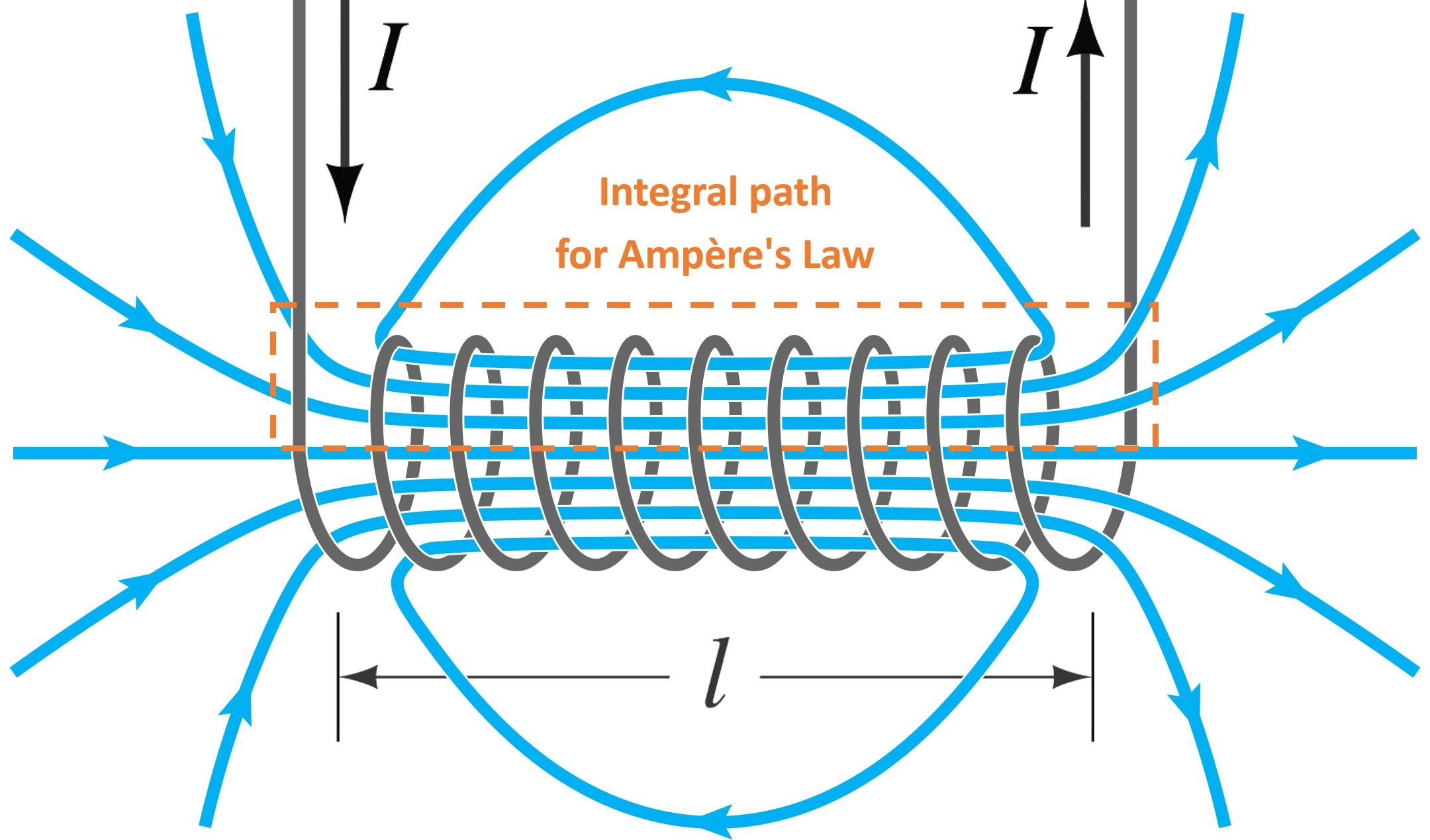
Solenoid creates a longitudinal magnetic field. It has a constant field inside the magnet, the field decreases to zero when sufficiently far from the magnet.
import numpy as np
import matplotlib.pyplot as plt

npoint=10000
sharpness=10
longilist=np.linspace(-6,6,npoint)
field=0*longilist
field[:npoint//2]=(np.arctan((longilist[:npoint//2]+3.5)*sharpness))/np.pi+0.5
field[npoint//2:]=np.flip(field[:npoint//2])
fig,ax=plt.subplots()
ax.plot(longilist, field, label='Realistic field')
ax.set_xlim(-6,6)
ax.set_ylim(0,1)
intb2=np.sum(field*field)
intb=np.sum(field)
hb=intb2/intb
hl=intb/hb*(longilist[1]-longilist[0])

ax.axvline(x=hl/2, ymin=0,ymax=hb,color='C1')
ax.axvline(x=-hl/2, ymin=0,ymax=hb,color='C1')
ax.axhline(y=hb, xmin=(-hl/2+6)/12,xmax=(hl/2+6)/12,color='C1',label='Hardedge approximation')
ax.legend()

The linear map of solenoid has to involve 4 dimensional coordinates $(x, x', y, y')$. Suppose a hard-edge model of solenoid with field $B_{\parallel}$ and length $L_0$. The rotation angle is
\begin{equation} \theta_s=\frac{eB_{\parallel}L_0}{2P_0}\equiv g_s L_0 \end{equation}Here, $g_s$ is defined as the relative solenoid strength.
\begin{equation} g_s\equiv \frac{eB_{\parallel}}{2P_0} \end{equation}The linear effect of the solenoid can be calculated as two dual-direction focusing elements, separated by a rotation.
\begin{equation} \left[\begin{array}{c} x\\ x'\\ y\\ y' \end{array}\right]_{f}=M_{sol}\left[\begin{array}{c} x\\ x'\\ y\\ y' \end{array}\right]_{i} \end{equation}where
\begin{align} M_{sol}&= \left[\begin{matrix}\cos^{2}{\left(\theta_{s}\right)} & \frac{\sin{\left(2\theta_{s}\right)}}{2g_{s}} & -\frac{\sin{\left(2\theta_{s}\right)}}{2} & -\frac{\sin^{2}{\left(\theta_{s}\right)}}{g_{s}}\\ -\frac{g_{s}\sin{\left(2\theta_{s}\right)}}{2} & \cos^{2}{\left(\theta_{s}\right)} & g_{s}\sin^{2}{\left(\theta_{s}\right)} & -\frac{\sin{\left(2\theta_{s}\right)}}{2}\\ \frac{\sin{\left(2\theta_{s}\right)}}{2} & \frac{\sin^{2}{\left(\theta_{s}\right)}}{g_{s}} & \cos^{2}{\left(\theta_{s}\right)} & \frac{\sin{\left(2\theta_{s}\right)}}{2g_{s}}\\ -g_{s}\sin^{2}{\left(\theta_{s}\right)} & \frac{\sin{\left(2\theta_{s}\right)}}{2} & -\frac{g_{s}\sin{\left(2\theta_{s}\right)}}{2} & \cos^{2}{\left(\theta_{s}\right)} \end{matrix}\right] \\ &=M_\text{focus}M_\text{rotation}M_\text{focus} \end{align}in which,
\begin{equation} M_\text{focus}=\left[\begin{matrix}\cos{\left(\frac{\theta_{s}}{2}\right)} & \frac{1}{g_{s}}\sin{\left(\frac{\theta_{s}}{2}\right)} & 0 & 0\\ -g_{s}\sin{\left(\frac{\theta_{s}}{2}\right)} & \cos{\left(\frac{\theta_{s}}{2}\right)} & 0 & 0\\ 0 & 0 & \cos{\left(\frac{\theta_{s}}{2}\right)} & \frac{1}{g_{s}}\sin{\left(\frac{\theta_{s}}{2}\right)}\\ 0 & 0 & -g_{s}\sin{\left(\frac{\theta_{s}}{2}\right)} & \cos{\left(\frac{\theta_{s}}{2}\right)} \end{matrix}\right] \end{equation}\begin{equation} M_\text{rotation}=\left[\begin{matrix}\cos{\left(\theta_s \right)} & 0 & - \sin{\left(\theta_s \right)} & 0\\0 & \cos{\left(\theta_s \right)} & 0 & - \sin{\left(\theta_s \right)}\\\sin{\left(\theta_s \right)} & 0 & \cos{\left(\theta_s \right)} & 0\\0 & \sin{\left(\theta_s \right)} & 0 & \cos{\left(\theta_s \right)}\end{matrix}\right] \end{equation}Intro to Dispersion and Chromaticity
Dispersion function
When particle has different energy (called off-momentum particle) than reference energy (correspond to the rigidity $B\rho$), two effects on the orbit rise.
First, the dipole will bend the particle differently, as shown in the below figure:
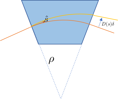
The corresponding Hill's equation reads:
\begin{equation} x''+\left(\frac{1}{\rho^2}+k(s)\right)x=\frac{\delta}{\rho} \end{equation}We define the dispersion assuming $x=x_\beta+ D \delta$, with $\delta$ as a energy parameter $\delta=(P-P_0)/P_0$. Then the dispersion is defined as:
\begin{equation} D(s)=\frac{dx(s)}{d\delta} \end{equation}which satisfy the same inhomogeneous differential equation:
\begin{equation} D''+\left(\frac{1}{\rho^2}+k(s)\right)D=\frac{1}{\rho} \end{equation}Therefore the dispersion function follows the same differential equation with source $1/\rho$, which is coming from a dipole magnet. The quadrupole does not 'create' dispersion but modifies it. The calculation of the dispersion will be covered in accelerator physics courses.
A direct consequence of dispersive effect is that the path length depends on the energy deviation.
\begin{equation} \frac{\Delta C}{C}=\frac{1}{C}\int\frac{D(s)\delta}{\rho}ds\equiv\alpha_C \delta \end{equation}Here, $\alpha_C$ is named momentum compaction factor. The energy difference not only causes the difference in pass length, but also in the traveling time:
Here, $\eta$ is the phase-slip factor.
Chromaticity
Another effect for an off-momentum particle is that the focal length of the quadrupole changes. Consequently, the phase advance of the lattice varies as the momentum of the particle changes. We will define the linear chromaticity $\xi$ as:
\begin{equation} \xi=\frac{d\nu}{d\delta} \end{equation}Both dispersion and chromaticity are inevitable since there is always dipoles and quadrupoles in the lattice. Many beam dynamics problems rise from them. Therefore the control of dispersion and chromaticity is essential component in accelerator design. We need to use sextrupoles to correct the chromaticity. However, the sextrupoles introduces nonlinearity in the system and requires attention of maintaining a large enough stable region.
import numpy as np
import matplotlib.pyplot as plt
from matplotlib import cm
num_par=500
xsize=0.8  # mm
pxsize=0.04 # mrad
coor=0
distance=1
focallen=-0.7
espread=0.2


step=2
dot_size_scale=np.log(2*num_par)**1.2
mod_xsize=xsize/np.sqrt(1+coor*coor)
beta=mod_xsize/pxsize
virtual_drift=coor*beta

espread_list=(np.random.rand(num_par)-0.5)*2*espread
emax=np.max(espread_list)
emin=np.min(espread_list)
colors=plt.cm.bwr((espread_list-emin)/(emax-emin))
particle_coor=np.zeros((3*step+3, num_par))
particle_coor[0, :]=np.random.randn(num_par)*mod_xsize
particle_coor[1, :]=np.random.randn(num_par)*pxsize
particle_coor[0, :]+=particle_coor[1, :]*virtual_drift
particle_coor[2, :]=np.zeros(num_par)-1.0

particle_coor[3, :]=particle_coor[0, :]+particle_coor[1, :]*distance
particle_coor[4, :]=particle_coor[1, :]
particle_coor[5, :]=particle_coor[2, :]+distance


particle_coor[7, :]=particle_coor[4, :]+particle_coor[3, :]/focallen/(1+espread_list)
particle_coor[6, :]=particle_coor[3, :]+particle_coor[7, :]*distance

particle_coor[8, :]=particle_coor[5,:]+distance

max_x=np.max([np.max(particle_coor[[0,3,6], :])*1.1, 3*xsize])
max_px=np.max([np.max(particle_coor[[1,4,7], :])*1.1, 3*pxsize])
fig,ax=plt.subplots(figsize=(8,6))
ax.set_xlim(-1.5,1.5)
ax.set_ylim(-max_x,max_x*1.6)
for i in range(num_par):
    ax.plot(particle_coor[[2,5,8],i],particle_coor[[0,3,6],i], lw=2/dot_size_scale, color=colors[i],)
ax.axvline(x=1,ymin=2/2.6-0.2, ymax=2/2.6, linestyle='-.', lw=1, alpha=.6)
ax.axvline(x=0,ymin=2/2.6-0.2, ymax=2/2.6, linestyle='-.', lw=1, alpha=.6)
ax.axvline(x=-1,ymin=2/2.6-0.2, ymax=2/2.6, linestyle='-.', lw=1, alpha=.6)
ax.set_xlabel("Longitudinal position [m]")
ax.set_ylabel("Transverse position [mm]")
axins1 = ax.inset_axes([0.02, 0.68, 0.3, 0.3])
axins1.set_xlim([-max_x,max_x])
axins1.set_ylim([-max_px,max_px])
axins1.plot(particle_coor[0,:], particle_coor[1,:],ls='None',marker='.', ms=6/dot_size_scale)
axins1.set_xticks([])
axins1.set_yticks([])

axins2 = ax.inset_axes([0.35, 0.68, 0.3, 0.3])
axins2.plot(particle_coor[3,:], particle_coor[4,:],ls='None',marker='.', ms=6/dot_size_scale)
axins2.set_xlim([-max_x,max_x])
axins2.set_ylim([-max_px,max_px])
axins2.set_xticks([])
axins2.set_yticks([])

axins3 = ax.inset_axes([0.68, 0.68, 0.3, 0.3])
axins3.plot(particle_coor[6,:], particle_coor[7,:],ls='None',marker='.', ms=6/dot_size_scale)
axins3.set_xlim([-max_x,max_x])
axins3.set_ylim([-max_px,max_px])
axins3.set_xticks([])
axins3.set_yticks([])
plt.show()
